6 - Morphological features extraction
Description: This notebook contains an example on how to read SRX localization data (in csv format) and extract morphological features to describe the shape of the trace.
These features together with descriptive statistics (number of localizations, mean position, mean precision, etc.) can be used to categorize individual segments.
The following index has links to the different sections of the notebook. Some sections may have additional indexes to access the subparts.
If you are using VS Code to visualize the notebook, the links will not work. This is due to how VC Code render the notebook. To navigate the notebook use the outline panel. To know more about it, check this link.
Content:
Library imports and functions
import re
from pathlib import Path

import numpy as np
import matplotlib.pyplot as plt
from matplotlib.colors import LinearSegmentedColormap
from matplotlib import colormaps
import seaborn as sns
import pandas as pd
from scipy.stats import mannwhitneyu, median_abs_deviation

from cima.parsers.parser_csv import CSVParser
from cima.utils.walk_features import getSegmentsFeatures
from cima.utils.stats_function import statConvert

# Set the maximum number of rows to display in the output
pd.options.display.max_rows = 999

# Set the options for saving the plots
plot_opts = {"dpi": 300, "bbox_inches": 'tight', "transparent": True}

# Labels for the plots of the features, so they look nice
plot_labels={
    "volume":"Volume ($nm^3$)",
    "area":"Area ($nm^2$)",
    "sphericity":"Sphericity",
    "sphericity_bribiesca":"Sphericity Bribiesca",
    "density_kb":"Density (blink/bp)",
    "density":"Density (blink/$nm^3$)",
    "compaction":"Genomic compactness (bp/$nm^3$)",
    "solidity":"Solidity",
    "radius_of_gyration":"Radius of gyration",
    "point_cloud_ellipticity":"Ellipticity",
    "numerosity":"Numerosity"
    }

# When showing dataframes we want that this are the first columns, so the user can manually search for them (not recomended)
first_cols = ["experimentID", "nucleusID", "chromosome", "homolog", "timepoint", "name", "flag"]

## Regular expressions to get the metadata from the filename
regex_patterns = {
    "nucleusID": re.compile(r"(?i)nuc(\d+)"), # This searches for "Nuc" or "nuc" followed by digits
    "cellID": re.compile(r"(?i)cell(\d+)"), # This searches for "Cell" or "cell" followed by digits
    "locationID" : re.compile(r"(?i)loc-?(\d+)"), # This searches for "Loc" or "loc" followed by optional hyphen and digits
    "date" : re.compile(r"(\d{4}[-\.]\d{2}[-\.]\d{2})"), # This searches for dates in the format YYYY-MM-DD or YYYY.MM.DD
    "homolog" : re.compile(r"_([ABPM01pm])"), ## Added just in case the homolog is in the filename.
    "chromosome" : re.compile(r"(?i)(chr[\d+MXY])") ## Added just in case the chromosome is in the filename.
    }

# Dictionary to change all the data types of the columns of the different dataframes, so the notebook is mor memory
# efficient.
dtype_dict = {
    "experimentID" : "string", "nucleusID" : "string", "chromosome" : "string",
    "homolog" : "string", "timepoint" : np.int16, "Name" :  "string", "flag" : "string", "segment1" : np.int16,
    "segment1_timepoint" : np.int16, "segment2_name" : "string", "flag_seg1" : "string", "segment2" : np.int16,
    "segment2_timepoint" : np.int16, "segment2_name" : "string", "flag_seg2" : "string", "coms_distance" : np.float32,
    "surface_distance" : np.float32, "entanglement" : np.float32, "volume" : np.float32,
    "area" : np.float32, "sphericity_bribiesca" : np.float32, "sphericity" : np.float32, "radius_of_gyration" : np.float32,
    "point_cloud_ellipticity" : np.float32, "point_cloud_eccentricity" : np.float32, "mvee_ellipticity" : np.float32,
    "mvee_eccentricity" : np.float32, "solidity" : np.float32, "holeless_solidity" : np.float32,
    "numerosity" : np.uint32, "compaction" : np.float32, "density" : np.float32, "density_kb" : np.float32
}

# We create a color map that goes from white to red for the HiC plots (put it in CIMA)
if "bright_red" not in colormaps:
    colormaps.register(name="bright_red", cmap=LinearSegmentedColormap.from_list("bright_red", [(1,1,1),(1,0,0)]))
# Function to batch process morphological features
def Batch_process_morphological_features(obj_list: list,
                        dataframe_genomic_info: pd.DataFrame,
                        size_column: str = "Size(kb)",
                        stepname_column: str = "timepoint",
                        library_n_Hype: int = 16,
                        metaInfo: list[str] = ["experimentID","nucleus","homolog"],
                        features2skip: list[str] = ["timepoint", "numerosity", "sphericity_bribiesca"],
                        prec_mean: float = 50.0,
                        ncores: int = 1) -> pd.DataFrame:

    """
    Processes a list of objects to get the morphological features of each timepoint/genomic segment.

    Parameters
    ----------
    obj_list : list
        List of objects to process.
    dataframe_genomic_info : pd.DataFrame
        DataFrame containing genomic information.
    size_column : str, optional
        Name of the column in dataframe_genomic_info that contains the size information (default is "Size(kb)").
    stepname_column : str, optional
        Name of the column in dataframe_genomic_info that contains the step names (default is "timepoint").
    library_n_Hype : int, optional
        Maximum number of segments allowed (default is 16).
    metaInfo : list[str], optional
        List of metadata keys to extract from each object (default is ["experimentID","nucleus","homolog"]).
    features2skip : list[str], optional
        List of feature names to skip (default is ["timepoint", "numerosity", "sphericity_bribiesca"]). Timepoint is skipped to avoid having to columns with the same name.
    prec_mean : float, optional
        Precision mean value (default is 50.0).
    ncores : int, optional
        Number of cores to use for parallel processing (default is 1).

    Returns
    -------
    pd.DataFrame
        DataFrame containing the morphological features for each timepoint/genomic segment.
    """

    import warnings
    warnings.filterwarnings("ignore", category=RuntimeWarning)
    # This is done to avoid a RuntimeWarning that happens in the GetEccentricity function. I reactivate it at the end of the loop.

    print(f"Calculating morphological features for {len(obj_list)} objects...")

    info_df_list=[]

    if "timepoint" not in features2skip:
        features2skip.append("timepoint")

    for obj_counter, obj in enumerate(obj_list, start = 1):

        experiment_id = obj.metadata[metaInfo[0]]
        nucleus_ID = obj.metadata[metaInfo[1]]
        homolog = obj.metadata[metaInfo[2]]
        nSteps=obj.no_of_Times()

        print(f"\033[1;4m\tProcessing file experimentID: {experiment_id}, nucleusID: {nucleus_ID}, homolog: {homolog} ({obj_counter}/{len(obj_list)}).\033[0m")

        if nSteps>library_n_Hype:
            print(f"\tWarning too many segment {nSteps} in experimentID: {experiment_id}, nucleusID: {nucleus_ID}, homolog: {homolog}")
            pass
        else:

            list_CS=obj.split_into_time(return_list = True)

            dataframe_features=getSegmentsFeatures(list_CS, prec_mean=prec_mean, verbose=False, n_jobs = ncores)

            info_from_walk=pd.DataFrame({
                "timepoint" : [cs.atomList.timepoint.unique()[0] for cs in list_CS],
                "experimentID" : [experiment_id] * len(list_CS),
                "nucleusID" : [nucleus_ID] * len(list_CS),
                "homolog" : [homolog] * len(list_CS)})

            features_dataframe=info_from_walk.merge(dataframe_genomic_info, left_on="timepoint", right_on = "timepoint").merge(dataframe_features,left_on="timepoint", right_on="timepoint")

            features_dataframe["flag"] = features_dataframe[["experimentID","nucleusID","homolog","timepoint"]].astype(str).apply('_'.join, axis=1)

            features_dataframe["compaction"] = features_dataframe[size_column] * 1000 / features_dataframe["volume"]
            features_dataframe["density"] = features_dataframe["numerosity"] / features_dataframe["volume"]
            features_dataframe["density_kb"] = features_dataframe["numerosity"] / features_dataframe[size_column] * 1000

            features_dataframe = features_dataframe[["experimentID", "nucleusID", "homolog", "timepoint", stepname_column, "flag"] +
                                                    [col for col in dataframe_features.columns if col not in features2skip] +
                                                    ["compaction", "density", "density_kb"]]

            info_df_list.append(features_dataframe)

    print("Creating the final DataFrame with all the morphological features for the different timepoints across experiments")
    dataframe_final_morph = pd.concat(info_df_list, ignore_index=True)

    warnings.filterwarnings("default", category=RuntimeWarning)

    print("Morphological features calculation completed.")

    return dataframe_final_morph
Setting some variables
In the following cell you should set up some variables for the script to run properly. Change the variables at your convenience, and then you can press “Run all” in the Jupyter Notebook.
Brief explanation of the different variables:
- work_folder: this variable is where the plots and the tsv files that the script creates will be stored.
- data_file: this variable is where the csv files to be assessed are stored.
- info_file: file that contains information about your walks, such as the chromosome, start and end of the steps. You need a columns that matches the 'timepoint' column in the csv files, to be able to show proper information.
- column_round: the column that matches the 'timepoint' column in the csv files.
- column_name: the column with the "nice" name for the steps. This will be used instead of the timepoint number. Use "" in case the information file does not have this column (in this case the name of the steps will be in the form of 'StepN' where N is an incremental number form 1 to the max number of steps).
- column_size: the column for the size of the segment. Use "" in case the information file does not have this column (in this case the notebook will calculate the size automatically of the segments according to the start and end positions in the file).
- column_start_pos: the column of the start position of the timepoint.
- column_end_pos: the column of the start position of the timepoint.
- number_of_steps: the number of steps in your library.
- starting_step: the step at which analysis should start.
- prec_mean_dataset: the worst precision of the three axes (usually the Z). This will be used as a blurring factor when creating the 3D maps to calculate the volumetric features.
- save_plots: save the plots into a folder or show them in the notebook.
- file_suffix: add a suffix to the different files created, in case you wish to save the results from different assessments in the same folder. It will be added as "_suffix" before the .tsv/.pdf.
The notebook will create a folder in the work_folder path called 6_morphological_features_extraction. Inside this folder 2 subfolders will be created, one for tsvs and one for plots. Inside each folder, a sub-subfolder with the suffix name will have the plots/tsvs for that experiment.
6_morphological_features_extraction/
|-- tsvs/
|   |-- example_tsv_SUFFIX.tsv
|-- plots/
|   |-- example_plot_SUFFIX.pdf
work_folder = "/scratch/CIMA_tutorial/"
data_folder = "/scratch/CIMA_tutorial/data/chr3"

info_file = "/scratch/CIMA_tutorial/data/chr3/Info_chr3.txt"
column_round = "Round"
column_name = "Name"
column_size = "Size(kb)"
column_chr = "Chr"
column_start_pos = "Start(hg19)"
column_end_pos = "End(hg19)"

number_of_steps_library = 16
starting_step = 6

prec_mean_dataset = 30

save_plots = False

file_suffix = "chr3"
work_folder = Path(work_folder)
data_folder = Path(data_folder)
pre_assessment_folder = Path(work_folder, "2_experimental_quality_assessment")
reconstruction_tsv_folder = Path(work_folder, "3_3D_reconstruction_assessment", "tsvs", file_suffix)

info_df = pd.read_table(Path(info_file), sep="\t")
info_df.columns = info_df.columns.str.strip() # In case there are leading or trailing spaces in the column names

info_file_dict = {
    "column_round" : column_round,
    "column_name" : column_name,
    "column_size" : column_size,
    "column_chr" : column_chr,
    "column_start_pos" : column_start_pos,
    "column_end_pos" : column_end_pos,
}

del column_round, column_name, column_size, column_chr, column_start_pos, column_end_pos, info_file
Exporting the data with CIMA
Content:
Creating the list of CIMA StructuralObject
In this cell we create a list of StructuralObjects (the main CIMA class type).
This list is the basis to do the assessment through this Jupyter Notebook.
When loading the data, we will also take out those traces or CS that did not pass the assessment in the previous notebooks.
When reading the file, it will also add some metadata gathered from the filename of the csv file:
- nucleusID: searches for "nuc" (with any combination of lower and upper case) followed by digits. If there is not a match, the default is filecount (first file read will be number 1, ...).
- cellID: searches for "cell" (with any combination of lower and upper case) followed by digits. If there is not a match, the default is filecount (first file read will be number 1, ...).
- locationID: searches for "loc" (with any combination of lower and upper case) followed by optional hyphen and digits.If there is not a match, the default is filecount (first file read will be number 1, ...).
- date: searches for dates in the format YYYY-MM-DD or YYYY.MM.DD. If there is not a match, the default is the file name.
- homolog: searches for "_" followed by A, B, M, P, m, p, 0 or 1 (only one instance of this). If there is not a match, the default is "A".
- chromosome: searches for "chr" (with any combination of lower and upper case) followed by a number, M, X or Y. If there is not a match, the default is "chrN".
# Get a list of all CSV files in the specified data folder
csv_files = list(data_folder.glob('*.csv'))

if len(csv_files) == 0:
    print("No files found, please input the correct work_folder")
else:
    print(f"Total number of files found: {len(csv_files)}")

print("Loading the experimental quality data from the CSV files")
traces_pass = pd.read_csv(Path(pre_assessment_folder, f"experimental_assessment_pass_{file_suffix}.txt"), sep="\t", names=["trace"])

print("Loading the bad flags from the CSV files")
segments_to_remove_CCC = pd.read_csv(Path(reconstruction_tsv_folder, f'segments2remove_bycccvariation_t2{("_" + file_suffix) if file_suffix != "" else ""}.tsv'), sep="\t")
if "flag" not in segments_to_remove_CCC.columns and not segments_to_remove_CCC.empty:
    print("\tCreating the 'flag' column for reconstruction-based removal")
    segments_to_remove_CCC["flag"] = segments_to_remove_CCC[["experimentID", "nucleusID", "homolog", "timepoint"]].astype(str).apply("_".join, axis=1)
    bad_flags = set(segments_to_remove_CCC["flag"].astype(str).values)
elif not segments_to_remove_CCC.empty:
    bad_flags = set(segments_to_remove_CCC["flag"].astype(str).values)
else:
    bad_flags = set()

# Get a list of metadata keys to extract from filenames
metadata_keys = ["nucleusID", "cellID", "locationID", "date", "homolog", "chromosome"]

# Initialize an empty list to store the StructuralObject instances
obj_list = []

if len(csv_files) > 0:
    # Iterate over each file in the list of file names
    for count, filein in enumerate(csv_files, start=1):

        stem = Path(filein).stem

        if not stem in traces_pass["trace"].values:
            print(f"Skipping file {count}: {stem} because it did not pass the experimental quality assessment.")
            continue

        print(f"Processing file {count}: {stem}", end="\r")

        # We mine the metadata from the filename using regex patterns. If not possible, assign default values.
        # In the case of nucleus, cell and location, the default is the filecount (first file read will be number 1, ...)
        # In the case of date, if no date can be found, the filename gets used.
        # If no valid homolog denomination is found, the default value is A.
        # If no valid chromosome denomination is found, the default value is chrN.
        metadata_CIMA = {
            key: (match.group(1) if (match := regex_patterns[key].search(stem)) else default)
            for key, default in zip(metadata_keys, [count, count, count, stem, "A", "chrN"])
        }

        # Adjust the metadata for nucleus and cell (if nucleus is count, but cell is something, use the cell match in nucleus)
        if "cellID" in metadata_CIMA and metadata_CIMA["nucleusID"] == count:
            metadata_CIMA["nucleusID"] = metadata_CIMA["cellID"]

        # Set experimentID as date for consistency
        metadata_CIMA["experimentID"] = metadata_CIMA["date"]

        # Read the CSV file and create a StructuralObject instance
        objin = CSVParser.read_CSV_file(filein.as_posix(), metadata = metadata_CIMA, content_type = "srx")

        # Filter the atomList to include only the specified timepoints in the info file
        objin.atomList = objin.atomList[(objin.atomList['timepoint'] >= starting_step - 1) &
                                        (objin.atomList['timepoint'] < (starting_step + number_of_steps_library - 1))].copy()

        experiment_id = objin.metadata["experimentID"]
        nucleus_id = int(objin.metadata["nucleusID"])
        homolog = objin.metadata["homolog"]

        full_flags = (experiment_id + "_" + str(nucleus_id) + "_" +homolog + "_" + objin.atomList["timepoint"].astype(str))
        remove_mask = full_flags.isin(bad_flags)

        if remove_mask.any():
            removed_tps = objin.atomList.loc[remove_mask, "timepoint"].unique()
            # removed_tps = ",".join([tp_names[tp] for tp in removed_tps])
            # print(f"Excluding timepoints {removed_tps} in experimentID: {experiment_id}, nucleusID: {nucleus_id}, homolog: {homolog} due to poor assessment.")
            objin.atomList = objin.atomList.loc[~remove_mask].copy()

        for tp in objin.atomList["timepoint"].unique():
            # Take out the timepoint from the atomList if it has less tha 10 points
            tp_mask = objin.atomList["timepoint"] == tp
            if tp_mask.sum() < 10:
                print(f"\tExcluding timepoint {tp} in experimentID: {experiment_id}, nucleusID: {nucleus_id}, homolog: {homolog} because it has less than 10 points.")
                objin.atomList = objin.atomList.loc[~tp_mask].copy()

        # Append the object to the list
        obj_list.append(objin)

    # Nice print to tell the user the number of objects created.
    print(f"\nTotal number of objects created: {len(obj_list)}")

    # Clean up memory by deleting some of the variables no longer needed
    del count, filein, stem, metadata_CIMA, match, objin

del csv_files, metadata_keys
del bad_flags
del experiment_id, nucleus_id, homolog, full_flags, remove_mask
if 'segments_to_remove_precision' in locals():
    del segments_to_remove_CCC
Total number of files found: 33
Loading the experimental quality data from the CSV files
Loading the bad flags from the CSV files
	Creating the 'flag' column for reconstruction-based removal
Skipping file 2: 2018-07-10_nuc04_A_chr3 because it did not pass the experimental quality assessment.
Skipping file 5: 2018-07-10_nuc03_A_chr3 because it did not pass the experimental quality assessment.
	Excluding timepoint 19 in experimentID: 2018-09-04, nucleusID: 7, homolog: A because it has less than 10 points.
Skipping file 26: 2018-09-04_nuc01_A_chr3 because it did not pass the experimental quality assessment.
Processing file 33: 2018-09-04_nuc06_A_chr3
Total number of objects created: 30
Checking the information file
This cells makes an adjustment in the info_df.
It checks if the column of the info_df that we will use as the link between this data frame and our walks has the same timepoints. This happens because most programs start with timepoint 0, while most information files start at timepoint 1.
This will create a new column in the dataframe that is called ‘timepoint’. This column will be modified so it has the same range as the timepoint column from the csv files.
list_of_timepoints = sorted({int(tp) for obj in obj_list for tp in obj.atomList.timepoint.unique()})
info_of_timepoints = list(map(int, info_df[info_file_dict["column_round"]].tolist()))

print(f'List of timepoints found across all objects: {list_of_timepoints}')
print(f'List of timepoints in the information file: {info_of_timepoints}\n')

if list_of_timepoints == info_of_timepoints:
    print('The timepoints found in the objects match those in the information file.')
    info_df["timepoint"] = info_df[info_file_dict["column_round"]]
elif set(list_of_timepoints).issubset(info_of_timepoints):
    print('Note: The timepoints found in the objects are a subset of those in the information file. Not all timepoints are present.')
    info_df["timepoint"] = info_df[info_file_dict["column_round"]]
elif list_of_timepoints == [x - 1 for x in info_of_timepoints]:
    print('Note: The column for the information file that has the timepoint is offset by 1 compared to the objects, adjusting accordingly.')
    info_df["timepoint"] = info_df[info_file_dict["column_round"]] - 1
elif set(list_of_timepoints).issubset({x - 1 for x in info_of_timepoints}):
    print('Note: The timepoints found in the objects are a subset of those in the information file, which are offset by 1 compared to the objects. Adjusting accordingly.')
    info_df["timepoint"] = info_df[info_file_dict["column_round"]] - 1
else:
    print('Warning: The timepoints found in the objects do not match those in the information file.')

if info_file_dict["column_size"] == "":
    print("Calculating size column from start and end positions...")
    column_size = "size"
    info_file_dict["column_size"] = column_size
    info_df[column_size] = info_df[info_file_dict["column_end_pos"]] - info_df[info_file_dict["column_start_pos"]]

if info_file_dict["column_name"] == "":
    print("Setting name column from round numbers...")
    info_file_dict["column_name"] = "name"
    info_df["name"] = [f"Step{i}" for i in range(1, info_df.shape[0]+1)]

tp_names = info_df.set_index("timepoint")[info_file_dict["column_name"]].to_dict()

del list_of_timepoints, info_of_timepoints
List of timepoints found across all objects: [5, 6, 7, 8, 9, 10, 11, 12, 13, 14, 15, 16, 17, 18, 19, 20]
List of timepoints in the information file: [6, 7, 8, 9, 10, 11, 12, 13, 14, 15, 16, 17, 18, 19, 20, 21]

Note: The column for the information file that has the timepoint is offset by 1 compared to the objects, adjusting accordingly.
Creating a color palette and the results folders for the tsv and plot files
Here we create a color palette automatically based on the different experiment ID found across the files. Experiment IDs are usually the date of the experiment. This allows to easily check for a possible batch effect.
We also create the folders were to store the results.
- 6_morphological_features_extraction/tsvs: a subfolder using the suffix name will be created, where the different tsv files will be stored.
- 6_morphological_features_extraction/plots: a subfolder using the suffix name will be created, where the different plots (in pdf format) will be stored.
# Define the color palette for experiments. Use the date or the experimentID (date) as the key.
color_palette = {exp_date: color for exp_date, color in zip(
    # We get a set of unique dates from the metadata of the objects
    set([file.metadata["experimentID"] for file in obj_list]),
    # We assign a color from the tab10 palette for each unique date
    sns.color_palette("tab10", n_colors=len(set([file.metadata["experimentID"] for file in obj_list])))
)}

# This palette is fixed for the current experiments used in the tutorial, which aim to reproduce the figures in the CIMA paper.
color_palette = {'2018-01-11':"#a6cee3" ,'2018-06-28':'#1f78b4', '2018-07-10':'#b2df8a', '2018-09-04':'#33a02c'}

# Create the folders to save the results. If the folders already exist, do not raise an error.
tsv_folder = Path(work_folder, "6_morphological_features_extraction", "tsvs", file_suffix)
tsv_folder.mkdir(parents=True, exist_ok=True)

plots_folder = Path(work_folder, "6_morphological_features_extraction", "plots", file_suffix)
plots_folder.mkdir(parents=True, exist_ok=True)
Extracting the morphological features
Content:
3D features calculation/loading
In this cell we check if the the morphological info has been calculated/loaded.
If it is not loaded (or it is not a pandas DataFrame), we try to load it from a file.
In case it said file does not exists it is calcualted, poorly assesed segments filtered out and saved.
if "features_3d_df" not in globals() or not isinstance(features_3d_df, pd.DataFrame):

    filename = f"morphological_features_{prec_mean_dataset}{('_' + file_suffix if file_suffix != '' else '')}.tsv"

    print("Trying to read pre-calculated morphological features from TSV file...")
    try:
        features_3d_df = pd.read_csv(Path(tsv_folder, filename), sep='\t')

        if "flag" not in features_3d_df.columns:
            features_3d_df["flag"] = features_3d_df[["experimentID","nucleusID","homolog","timepoint"]].astype(str).apply('_'.join, axis=1)

        print("Pre-calculated morphological features loaded from TSV file.")

    except FileNotFoundError:

        print("Pre-calculated TSV file not found. Calculating morphological features from scratch...")
        features_3d_df = Batch_process_morphological_features(
            obj_list = obj_list,
            dataframe_genomic_info = info_df,
            size_column = info_file_dict["column_size"],
            stepname_column=info_file_dict["column_name"],
            library_n_Hype = number_of_steps_library,
            metaInfo = ["experimentID","nucleusID","homolog"],
            features2skip = [],
            prec_mean = prec_mean_dataset,
            ncores = 1
        )

        print("Saving morphological features to TSV file...", end="\r")
        features_3d_df.drop(columns=["flag"]).to_csv(Path(tsv_folder, filename), sep='\t', index=False)
        print("Saving morphological features to TSV file... Done!")

        print("Morphological features calculated and saved to TSV file.")

    del filename

else:
    print("Morphological features DataFrame already exists in memory.")

if "flag2" not in features_3d_df.columns:
    features_3d_df["flag2"] = features_3d_df[["experimentID","nucleusID","homolog"]].astype(str).apply('_'.join, axis=1)

features_3d_df = features_3d_df.sort_values(by="timepoint")
display(features_3d_df.head())
Trying to read pre-calculated morphological features from TSV file...
Pre-calculated TSV file not found. Calculating morphological features from scratch...
Calculating morphological features for 30 objects...
	Processing file experimentID: 2018-09-04, nucleusID: 03, homolog: A (1/30).
	Processing file experimentID: 2018-07-10, nucleusID: 02, homolog: A (2/30).
	Processing file experimentID: 2018-07-10, nucleusID: 05, homolog: A (3/30).
	Processing file experimentID: 2018-06-28, nucleusID: 07, homolog: A (4/30).
	Processing file experimentID: 2018-06-28, nucleusID: 09, homolog: A (5/30).
	Processing file experimentID: 2018-07-10, nucleusID: 11, homolog: A (6/30).
	Processing file experimentID: 2018-09-04, nucleusID: 01, homolog: B (7/30).
	Processing file experimentID: 2018-07-10, nucleusID: 06, homolog: B (8/30).
	Processing file experimentID: 2018-06-28, nucleusID: 05, homolog: B (9/30).
	Processing file experimentID: 2018-07-10, nucleusID: 06, homolog: A (10/30).
	Processing file experimentID: 2018-06-28, nucleusID: 08, homolog: A (11/30).
	Processing file experimentID: 2018-06-28, nucleusID: 05, homolog: A (12/30).
	Processing file experimentID: 2018-07-10, nucleusID: 07, homolog: A (13/30).
	Processing file experimentID: 2018-07-10, nucleusID: 01, homolog: A (14/30).
	Processing file experimentID: 2018-07-10, nucleusID: 02, homolog: B (15/30).
	Processing file experimentID: 2018-06-28, nucleusID: 01, homolog: A (16/30).
	Processing file experimentID: 2018-09-04, nucleusID: 04, homolog: A (17/30).
	Processing file experimentID: 2018-07-10, nucleusID: 04, homolog: B (18/30).
	Processing file experimentID: 2018-09-04, nucleusID: 03, homolog: B (19/30).
	Processing file experimentID: 2018-07-10, nucleusID: 03, homolog: B (20/30).
	Processing file experimentID: 2018-07-10, nucleusID: 01, homolog: B (21/30).
	Processing file experimentID: 2018-09-04, nucleusID: 07, homolog: A (22/30).
	Processing file experimentID: 2018-06-28, nucleusID: 02, homolog: A (23/30).
	Processing file experimentID: 2018-07-10, nucleusID: 10, homolog: A (24/30).
	Processing file experimentID: 2018-07-10, nucleusID: 08, homolog: A (25/30).
	Processing file experimentID: 2018-09-04, nucleusID: 05, homolog: A (26/30).
	Processing file experimentID: 2018-06-28, nucleusID: 01, homolog: B (27/30).
	Processing file experimentID: 2018-09-04, nucleusID: 10, homolog: A (28/30).
	Processing file experimentID: 2018-06-28, nucleusID: 07, homolog: B (29/30).
	Processing file experimentID: 2018-09-04, nucleusID: 06, homolog: A (30/30).
Creating the final DataFrame with all the morphological features for the different timepoints across experiments
Morphological features calculation completed.
Saving morphological features to TSV file... Done!
Morphological features calculated and saved to TSV file.
| experimentID | nucleusID | homolog | timepoint | Name | flag | volume | area | sphericity_bribiesca | sphericity | ... | point_cloud_eccentricity | mvee_ellipticity | mvee_eccentricity | solidity | holeless_solidity | numerosity | compaction | density | density_kb | flag2 | |
|---|---|---|---|---|---|---|---|---|---|---|---|---|---|---|---|---|---|---|---|---|---|
| 73 | 2018-07-10 | 11 | A | 5 | Step1 | 2018-07-10_11_A_5 | 45549000.0 | 1.334969e+06 | 0.849249 | 0.462025 | ... | 0.631109 | 0.811229 | 0.681738 | 0.147928 | 0.147928 | 4029.0 | 0.010977 | 0.000088 | 8058.0 | 2018-07-10_11_A |
| 88 | 2018-09-04 | 01 | B | 5 | Step1 | 2018-09-04_01_B_5 | 56322000.0 | 1.477865e+06 | 0.875486 | 0.480804 | ... | 0.223474 | 0.786694 | 0.577798 | 0.338188 | 0.338188 | 7982.0 | 0.008878 | 0.000142 | 15964.0 | 2018-09-04_01_B |
| 363 | 2018-07-10 | 08 | A | 5 | Step1 | 2018-07-10_08_A_5 | 24165000.0 | 7.481200e+05 | 0.859796 | 0.540303 | ... | 0.287081 | 0.810575 | 0.723042 | 0.252932 | 0.252932 | 4138.0 | 0.020691 | 0.000171 | 8276.0 | 2018-07-10_08_A |
| 287 | 2018-07-10 | 03 | B | 5 | Step1 | 2018-07-10_03_B_5 | 85833000.0 | 2.267695e+06 | 0.864498 | 0.414956 | ... | 0.274333 | 0.679143 | 0.652617 | 0.218693 | 0.218693 | 8507.0 | 0.005825 | 0.000099 | 17014.0 | 2018-07-10_03_B |
| 256 | 2018-07-10 | 04 | B | 5 | Step1 | 2018-07-10_04_B_5 | 29268000.0 | 9.034645e+05 | 0.854050 | 0.508357 | ... | 0.205049 | 0.699012 | 0.601044 | 0.361997 | 0.361997 | 2320.0 | 0.017084 | 0.000079 | 4640.0 | 2018-07-10_04_B |
5 rows × 22 columns
Plot 3D feature per segment
Boxplots of the different morphological features calculated, separated by chromatin segment
labels = features_3d_df[info_file_dict["column_name"]].unique().astype(str).tolist()

features_3d_df = features_3d_df[features_3d_df["point_cloud_ellipticity"] <= 0.8].copy()

for feature in ["volume", "area", "density_kb",
                "sphericity_bribiesca", "sphericity", "radius_of_gyration",
                "point_cloud_ellipticity",  "solidity","compaction", "numerosity"]:

    print(feature.capitalize())

    plt.figure(figsize=(10,3))
    sns.boxplot(x = features_3d_df[info_file_dict["column_name"]],
                y = features_3d_df[feature],
                hue = features_3d_df[info_file_dict["column_name"]], palette="turbo")
    sns.stripplot(x = features_3d_df[info_file_dict["column_name"]], y = features_3d_df[feature],
                  color='grey', alpha = 0.5)

    plt.ylabel(plot_labels[feature])
    plt.xlabel("Walk segment #ID")
    plt.ticklabel_format(style='sci',axis="y",scilimits=(0,0))
    plt.xticks(ticks=range(len(labels)), labels=labels, rotation=45, ha="right")

    sns.despine()

    if save_plots:
        filename = f'boxplot_{feature}_segment' + (f"_{file_suffix}" if file_suffix != '' else '') + '.pdf'
        plot_filename = Path(plots_folder, filename)
        print(f"Saving plots to: {plot_filename}")
        plt.savefig(plot_filename, **plot_opts)
        del filename, plot_filename
    else:
        plt.show()
    plt.close()

    stats_df=[]
    all_val = [float(x) for x in features_3d_df[feature].tolist()]
    grps = features_3d_df[info_file_dict["column_name"]].unique()
    d_data = {grp:features_3d_df[features_3d_df[info_file_dict["column_name"]] == grp][feature].tolist() for grp in grps}

    for grp in grps:
        T,p=mannwhitneyu(all_val,d_data[grp])
        stats_df.append( [grp,f"{p:.2f}",statConvert(f"{p:.2f}")])

    stats_df=pd.DataFrame(stats_df,
                          columns=["Segment name","Mann-Whitney U p-value","converted p-value"])

    print("p-values of Mann-Whitney U test comparing each segment against all the others:")
    display(stats_df)
    print()

del feature, stats_df, all_val, grps, d_data, grp, T, p, labels
Volume
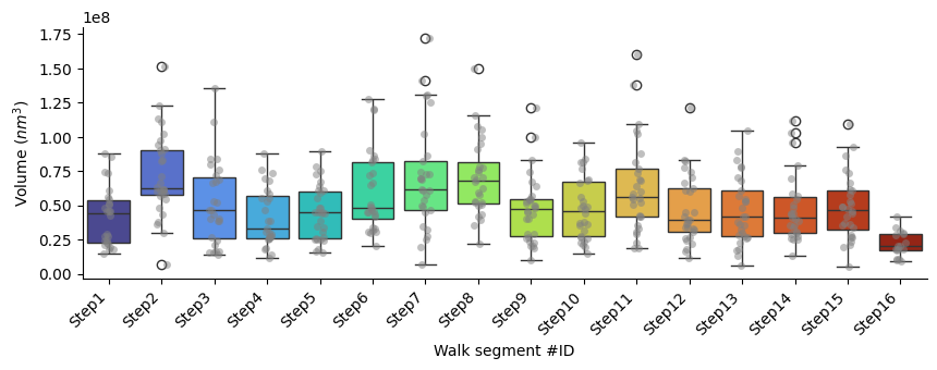
p-values of Mann-Whitney U test comparing each segment against all the others:
| Segment name | Mann-Whitney U p-value | converted p-value | |
|---|---|---|---|
| 0 | Step1 | 0.08 | 8.00E-2 |
| 1 | Step2 | 0.00 | **** |
| 2 | Step3 | 0.79 | 7.90E-1 |
| 3 | Step4 | 0.08 | 8.00E-2 |
| 4 | Step5 | 0.26 | 2.60E-1 |
| 5 | Step6 | 0.13 | 1.30E-1 |
| 6 | Step7 | 0.01 | ** |
| 7 | Step8 | 0.00 | **** |
| 8 | Step9 | 0.45 | 4.50E-1 |
| 9 | Step10 | 0.53 | 5.30E-1 |
| 10 | Step11 | 0.08 | 8.00E-2 |
| 11 | Step12 | 0.32 | 3.20E-1 |
| 12 | Step13 | 0.35 | 3.50E-1 |
| 13 | Step14 | 0.44 | 4.40E-1 |
| 14 | Step15 | 0.72 | 7.20E-1 |
| 15 | Step16 | 0.00 | **** |
Area
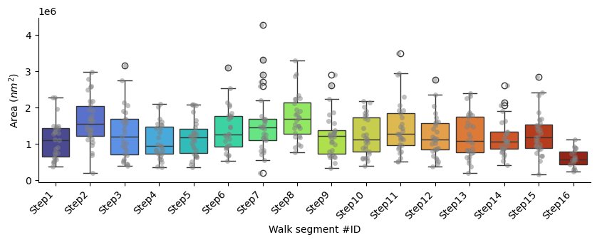
p-values of Mann-Whitney U test comparing each segment against all the others:
| Segment name | Mann-Whitney U p-value | converted p-value | |
|---|---|---|---|
| 0 | Step1 | 0.18 | 1.80E-1 |
| 1 | Step2 | 0.00 | **** |
| 2 | Step3 | 0.87 | 8.70E-1 |
| 3 | Step4 | 0.10 | 1.00E-1 |
| 4 | Step5 | 0.48 | 4.80E-1 |
| 5 | Step6 | 0.24 | 2.40E-1 |
| 6 | Step7 | 0.10 | 1.00E-1 |
| 7 | Step8 | 0.00 | **** |
| 8 | Step9 | 0.56 | 5.60E-1 |
| 9 | Step10 | 0.64 | 6.40E-1 |
| 10 | Step11 | 0.30 | 3.00E-1 |
| 11 | Step12 | 0.50 | 5.00E-1 |
| 12 | Step13 | 0.66 | 6.60E-1 |
| 13 | Step14 | 0.42 | 4.20E-1 |
| 14 | Step15 | 0.99 | 9.90E-1 |
| 15 | Step16 | 0.00 | **** |
Density_kb
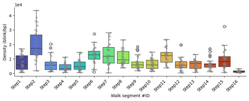
p-values of Mann-Whitney U test comparing each segment against all the others:
| Segment name | Mann-Whitney U p-value | converted p-value | |
|---|---|---|---|
| 0 | Step1 | 0.59 | 5.90E-1 |
| 1 | Step2 | 0.00 | **** |
| 2 | Step3 | 0.10 | 1.00E-1 |
| 3 | Step4 | 0.00 | **** |
| 4 | Step5 | 0.01 | ** |
| 5 | Step6 | 0.00 | **** |
| 6 | Step7 | 0.00 | **** |
| 7 | Step8 | 0.01 | ** |
| 8 | Step9 | 0.25 | 2.50E-1 |
| 9 | Step10 | 0.19 | 1.90E-1 |
| 10 | Step11 | 0.00 | **** |
| 11 | Step12 | 0.09 | 9.00E-2 |
| 12 | Step13 | 0.16 | 1.60E-1 |
| 13 | Step14 | 0.14 | 1.40E-1 |
| 14 | Step15 | 0.52 | 5.20E-1 |
| 15 | Step16 | 0.00 | **** |
Sphericity_bribiesca
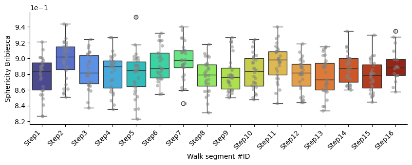
p-values of Mann-Whitney U test comparing each segment against all the others:
| Segment name | Mann-Whitney U p-value | converted p-value | |
|---|---|---|---|
| 0 | Step1 | 0.19 | 1.90E-1 |
| 1 | Step2 | 0.00 | **** |
| 2 | Step3 | 0.96 | 9.60E-1 |
| 3 | Step4 | 0.79 | 7.90E-1 |
| 4 | Step5 | 0.33 | 3.30E-1 |
| 5 | Step6 | 0.16 | 1.60E-1 |
| 6 | Step7 | 0.01 | ** |
| 7 | Step8 | 0.14 | 1.40E-1 |
| 8 | Step9 | 0.14 | 1.40E-1 |
| 9 | Step10 | 0.64 | 6.40E-1 |
| 10 | Step11 | 0.02 | * |
| 11 | Step12 | 0.22 | 2.20E-1 |
| 12 | Step13 | 0.17 | 1.70E-1 |
| 13 | Step14 | 0.75 | 7.50E-1 |
| 14 | Step15 | 0.09 | 9.00E-2 |
| 15 | Step16 | 0.40 | 4.00E-1 |
Sphericity
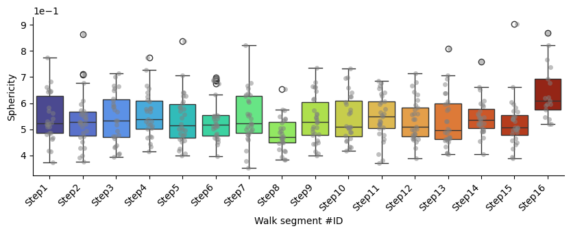
p-values of Mann-Whitney U test comparing each segment against all the others:
| Segment name | Mann-Whitney U p-value | converted p-value | |
|---|---|---|---|
| 0 | Step1 | 0.73 | 7.30E-1 |
| 1 | Step2 | 0.87 | 8.70E-1 |
| 2 | Step3 | 0.83 | 8.30E-1 |
| 3 | Step4 | 0.30 | 3.00E-1 |
| 4 | Step5 | 0.79 | 7.90E-1 |
| 5 | Step6 | 0.91 | 9.10E-1 |
| 6 | Step7 | 0.70 | 7.00E-1 |
| 7 | Step8 | 0.00 | **** |
| 8 | Step9 | 0.86 | 8.60E-1 |
| 9 | Step10 | 0.94 | 9.40E-1 |
| 10 | Step11 | 0.43 | 4.30E-1 |
| 11 | Step12 | 0.74 | 7.40E-1 |
| 12 | Step13 | 0.44 | 4.40E-1 |
| 13 | Step14 | 0.51 | 5.10E-1 |
| 14 | Step15 | 0.31 | 3.10E-1 |
| 15 | Step16 | 0.00 | **** |
Radius_of_gyration
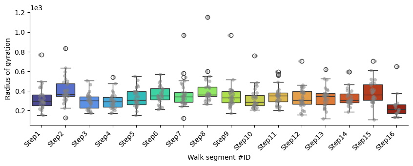
p-values of Mann-Whitney U test comparing each segment against all the others:
| Segment name | Mann-Whitney U p-value | converted p-value | |
|---|---|---|---|
| 0 | Step1 | 0.31 | 3.10E-1 |
| 1 | Step2 | 0.00 | **** |
| 2 | Step3 | 0.03 | * |
| 3 | Step4 | 0.03 | * |
| 4 | Step5 | 0.72 | 7.20E-1 |
| 5 | Step6 | 0.27 | 2.70E-1 |
| 6 | Step7 | 0.43 | 4.30E-1 |
| 7 | Step8 | 0.00 | **** |
| 8 | Step9 | 0.93 | 9.30E-1 |
| 9 | Step10 | 0.16 | 1.60E-1 |
| 10 | Step11 | 0.52 | 5.20E-1 |
| 11 | Step12 | 0.83 | 8.30E-1 |
| 12 | Step13 | 0.99 | 9.90E-1 |
| 13 | Step14 | 0.81 | 8.10E-1 |
| 14 | Step15 | 0.04 | * |
| 15 | Step16 | 0.00 | **** |
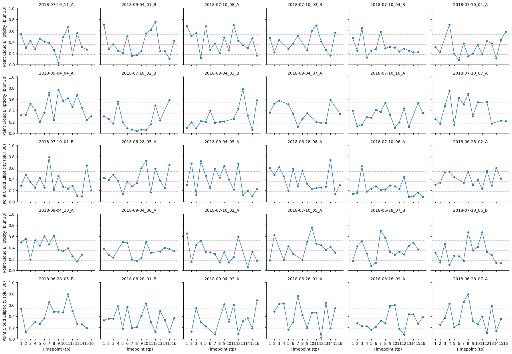
Point_cloud_ellipticity
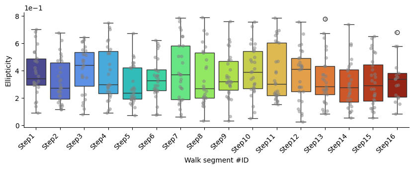
p-values of Mann-Whitney U test comparing each segment against all the others:
| Segment name | Mann-Whitney U p-value | converted p-value | |
|---|---|---|---|
| 0 | Step1 | 0.30 | 3.00E-1 |
| 1 | Step2 | 0.35 | 3.50E-1 |
| 2 | Step3 | 0.09 | 9.00E-2 |
| 3 | Step4 | 0.46 | 4.60E-1 |
| 4 | Step5 | 0.05 | * |
| 5 | Step6 | 0.98 | 9.80E-1 |
| 6 | Step7 | 0.49 | 4.90E-1 |
| 7 | Step8 | 0.67 | 6.70E-1 |
| 8 | Step9 | 0.67 | 6.70E-1 |
| 9 | Step10 | 0.15 | 1.50E-1 |
| 10 | Step11 | 0.75 | 7.50E-1 |
| 11 | Step12 | 0.65 | 6.50E-1 |
| 12 | Step13 | 0.53 | 5.30E-1 |
| 13 | Step14 | 0.13 | 1.30E-1 |
| 14 | Step15 | 0.33 | 3.30E-1 |
| 15 | Step16 | 0.74 | 7.40E-1 |
Solidity
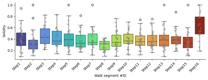
p-values of Mann-Whitney U test comparing each segment against all the others:
| Segment name | Mann-Whitney U p-value | converted p-value | |
|---|---|---|---|
| 0 | Step1 | 0.51 | 5.10E-1 |
| 1 | Step2 | 0.06 | 6.00E-2 |
| 2 | Step3 | 0.06 | 6.00E-2 |
| 3 | Step4 | 0.26 | 2.60E-1 |
| 4 | Step5 | 0.68 | 6.80E-1 |
| 5 | Step6 | 0.53 | 5.30E-1 |
| 6 | Step7 | 0.95 | 9.50E-1 |
| 7 | Step8 | 0.00 | **** |
| 8 | Step9 | 0.68 | 6.80E-1 |
| 9 | Step10 | 0.73 | 7.30E-1 |
| 10 | Step11 | 0.82 | 8.20E-1 |
| 11 | Step12 | 0.96 | 9.60E-1 |
| 12 | Step13 | 0.94 | 9.40E-1 |
| 13 | Step14 | 0.56 | 5.60E-1 |
| 14 | Step15 | 0.15 | 1.50E-1 |
| 15 | Step16 | 0.00 | **** |
Compaction
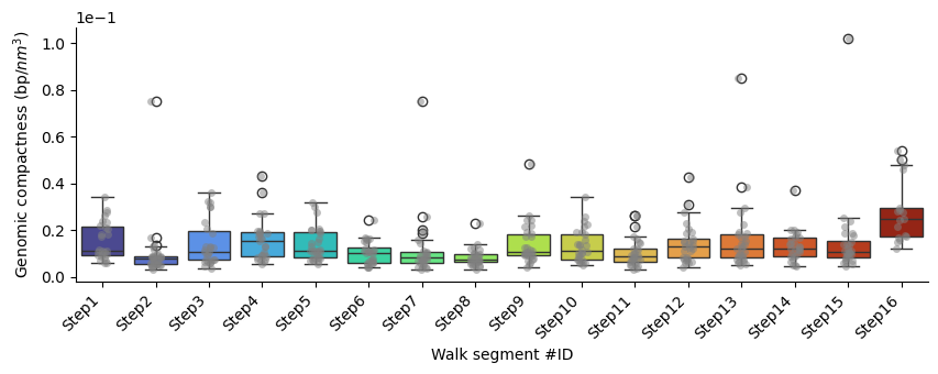
p-values of Mann-Whitney U test comparing each segment against all the others:
| Segment name | Mann-Whitney U p-value | converted p-value | |
|---|---|---|---|
| 0 | Step1 | 0.08 | 8.00E-2 |
| 1 | Step2 | 0.00 | **** |
| 2 | Step3 | 0.79 | 7.90E-1 |
| 3 | Step4 | 0.08 | 8.00E-2 |
| 4 | Step5 | 0.26 | 2.60E-1 |
| 5 | Step6 | 0.13 | 1.30E-1 |
| 6 | Step7 | 0.01 | ** |
| 7 | Step8 | 0.00 | **** |
| 8 | Step9 | 0.45 | 4.50E-1 |
| 9 | Step10 | 0.53 | 5.30E-1 |
| 10 | Step11 | 0.08 | 8.00E-2 |
| 11 | Step12 | 0.32 | 3.20E-1 |
| 12 | Step13 | 0.35 | 3.50E-1 |
| 13 | Step14 | 0.44 | 4.40E-1 |
| 14 | Step15 | 0.72 | 7.20E-1 |
| 15 | Step16 | 0.00 | **** |
Numerosity
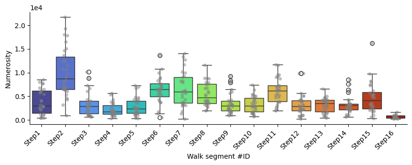
p-values of Mann-Whitney U test comparing each segment against all the others:
| Segment name | Mann-Whitney U p-value | converted p-value | |
|---|---|---|---|
| 0 | Step1 | 0.59 | 5.90E-1 |
| 1 | Step2 | 0.00 | **** |
| 2 | Step3 | 0.10 | 1.00E-1 |
| 3 | Step4 | 0.00 | **** |
| 4 | Step5 | 0.01 | ** |
| 5 | Step6 | 0.00 | **** |
| 6 | Step7 | 0.00 | **** |
| 7 | Step8 | 0.01 | ** |
| 8 | Step9 | 0.25 | 2.50E-1 |
| 9 | Step10 | 0.19 | 1.90E-1 |
| 10 | Step11 | 0.00 | **** |
| 11 | Step12 | 0.09 | 9.00E-2 |
| 12 | Step13 | 0.16 | 1.60E-1 |
| 13 | Step14 | 0.14 | 1.40E-1 |
| 14 | Step15 | 0.52 | 5.20E-1 |
| 15 | Step16 | 0.00 | **** |
feature2plot = "point_cloud_ellipticity"

mean_feature = features_3d_df[feature2plot].mean()
std_feature = features_3d_df[feature2plot].std()

g = sns.relplot(
        data=features_3d_df,
        x="timepoint",
        y=feature2plot,
        col="flag2",
        col_wrap=6,          # adjust as needed
        kind="line",
        marker="o",
        linewidth=1.2,
        height=2.5,
        aspect=1.2,
        facet_kws={"sharey": True, "sharex": True},
        # ylim = (0, 1)
    )

g.set_axis_labels("Timepoint (tp)", f"{feature2plot.replace('_', ' ').title()} (blur {prec_mean_dataset})")
g.set_titles("{col_name}")
g.set(ylim=(0,1))

for ax in g.axes.flat:
    x_min = int(features_3d_df["timepoint"].min())
    x_max = int(features_3d_df["timepoint"].max())
    ax.set_xticks(range(x_min, x_max + 1))
    ax.set_xticklabels(range(1, number_of_steps_library + 1))
    ax.grid(False)
    ax.axhline(mean_feature, color = "red", alpha = 0.25, zorder = 0)
    ax.axhline(mean_feature+std_feature, color = "black", alpha = 0.25, zorder = 0, linestyle="--")
    ax.axhline(mean_feature-std_feature, color = "black", alpha = 0.25, zorder = 0, linestyle="--")


plt.tight_layout()
if save_plots:
    filename = f'lineplot_{feature2plot}_pertrace' + (f"_{file_suffix}" if file_suffix != '' else '') + '.pdf'
    plot_filename = Path(plots_folder, filename)
    print(f"Saving plots to: {plot_filename}")
    plt.savefig(plot_filename, **plot_opts)
    del filename, plot_filename
else:
    plt.show()
plt.close()
plt.close()

del feature2plot, mean_feature, std_feature, g, ax, x_min, x_max
Distribution plot of compaction
Plot of the distribution for the compaction (bp/nm³) across the different timepoints and walks
sns.displot(x=features_3d_df["compaction"], kind="kde", fill=True)
plt.xlabel(plot_labels["compaction"])
plt.ylabel("Density")
plt.title("Distribution of Compaction")
sns.despine()
if save_plots:
    filename = f'distribution_of_compaction' + (f"_{file_suffix}" if file_suffix != '' else '') + '.pdf'
    plot_filename = Path(plots_folder, filename)
    print(f"Saving plots to: {plot_filename}")
    plt.savefig(plot_filename, **plot_opts)
    del filename, plot_filename
else:
    plt.show()
plt.close()

print(f"Max compaction over all the data: {np.max(features_3d_df['compaction'])}")
print(f"Min compaction over all the data: {np.min(features_3d_df['compaction'])}")
print(f"Median compaction over all the data: {np.nanmedian(features_3d_df['compaction'])}")
print(f"Median absolute deviation of compaction over all the data: {median_abs_deviation(features_3d_df['compaction'])}")
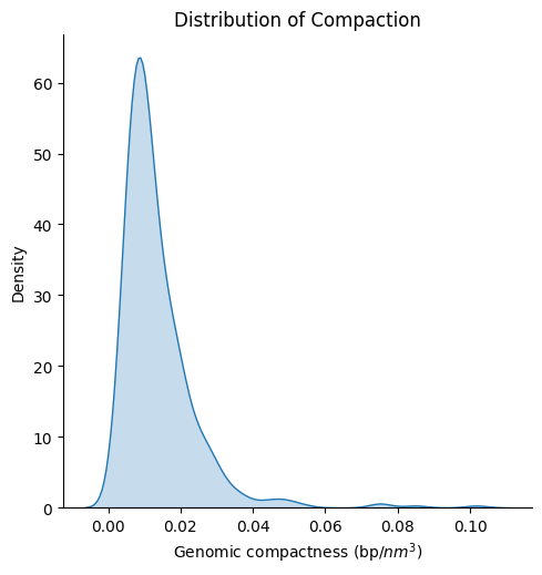
Max compaction over all the data: 0.10175010175010175
Min compaction over all the data: 0.0029094294608827207
Median compaction over all the data: 0.010513170439172999
Median absolute deviation of compaction over all the data: 0.003969821687193798
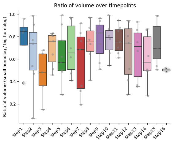
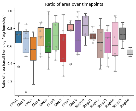
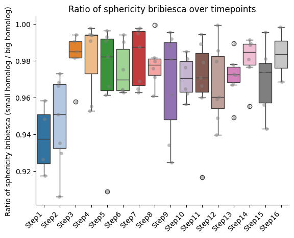
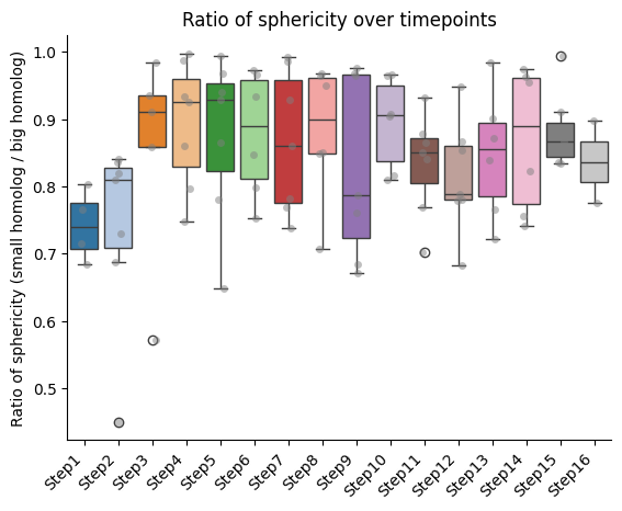
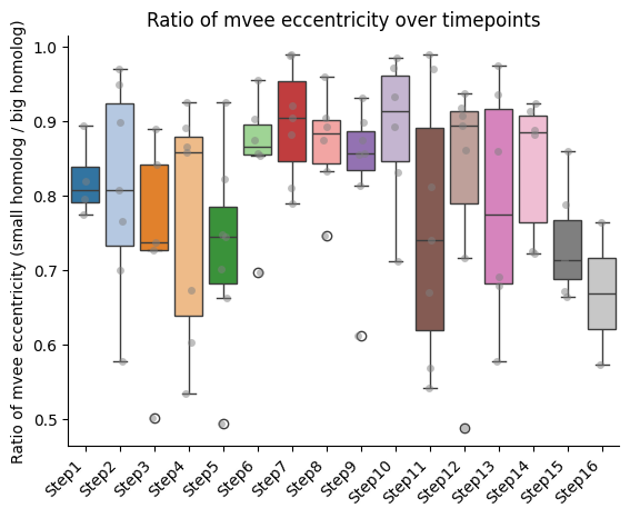
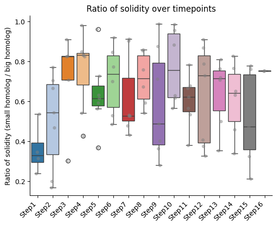
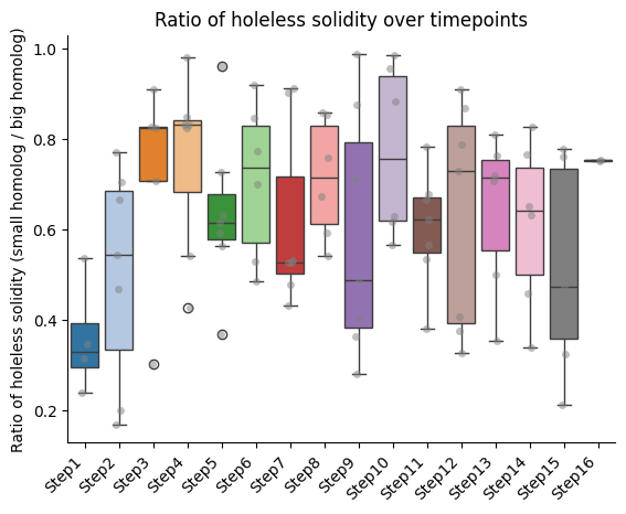
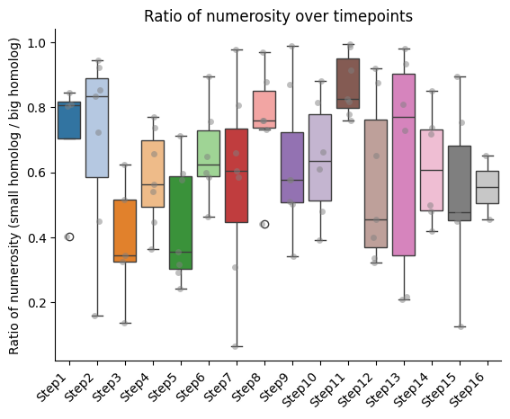
Ratios of features between homologs
Here we retrieve those walks for which we have the pair of homologs, and compute the ratio of the features between them.
IMPORTANT!!! The ratio is always calculated as smaller homolog divided by bigger homolog.
# TODO: to create a syntehtic dataset use Create_Random_Hom_Ratio_smalloverlarger

ratios2calculate = ['volume',
       'area', 'sphericity_bribiesca', 'sphericity', 'radius_of_gyration',
       'point_cloud_ellipticity', 'point_cloud_eccentricity',
       'mvee_ellipticity', 'mvee_eccentricity', 'solidity',
       'holeless_solidity', 'numerosity']

listratio=[]
both_homs_detected=0

for expID_nucID, group_rows in features_3d_df.groupby(["experimentID", "nucleusID"]):

    if len(group_rows.homolog.unique())==2:

        both_homs_detected+=1
        homA_df = group_rows[group_rows.homolog==group_rows.homolog.unique()[0]]
        homB_df = group_rows[group_rows.homolog==group_rows.homolog.unique()[1]]

        for tp in group_rows.timepoint.sort_values().unique():
            homA_step=homA_df[homA_df.timepoint == tp]
            homB_step=homB_df[homB_df.timepoint == tp]

            if len(homA_step!=0) and len(homB_step!=0):
                homA_step = homA_step[ratios2calculate].copy()
                homA_step.reset_index(drop=True, inplace=True)
                homA_step = homA_step.astype(float)

                homB_step = homB_step[ratios2calculate].copy()
                homB_step.reset_index(drop=True, inplace=True)
                homB_step = homB_step.astype(float)

                temp = pd.DataFrame()

                for feature in ratios2calculate:
                    if homA_step[feature].values[0] > homB_step[feature].values[0]:
                        homA_val = homA_step[feature].values[0]
                        homB_val = homB_step[feature].values[0]
                        ratio = homB_val / homA_val if homA_val != 0 else np.nan
                    else:
                        homA_val = homA_step[feature].values[0]
                        homB_val = homB_step[feature].values[0]
                        ratio = homA_val / homB_val if homB_val != 0 else np.nan
                    temp[feature] = [ratio]

                temp = temp.replace([np.inf, -np.inf], np.nan)

                temp["experimentID"] = expID_nucID[0]
                temp["nucleusID"] = expID_nucID[1]
                temp["timepoint"] = tp
                temp["name"] = tp_names[tp]
                temp["flag"] = f"{expID_nucID[0]}_{expID_nucID[1]}_{tp}"

                listratio.append(temp)

print(f"Number of nuclei with both homologs detected: {both_homs_detected}")
if both_homs_detected > 0:
    ratio_df = pd.concat(listratio, ignore_index=True)

    # Put experimentID, nucleusID, timepoint and flag columns as the first ones
    cols = ratio_df.columns.tolist()
    cols_reorder = [col for col in first_cols if col in cols] + [col for col in ratio_df.columns if col not in first_cols]
    ratio_df = ratio_df[cols_reorder]

    display(ratio_df.head())

del listratio, expID_nucID, group_rows
if both_homs_detected > 0:
    del homA_df, homB_df, tp, homA_step, homB_step, temp, cols, cols_reorder
Number of nuclei with both homologs detected: 7
| experimentID | nucleusID | timepoint | name | flag | volume | area | sphericity_bribiesca | sphericity | radius_of_gyration | point_cloud_ellipticity | point_cloud_eccentricity | mvee_ellipticity | mvee_eccentricity | solidity | holeless_solidity | numerosity | |
|---|---|---|---|---|---|---|---|---|---|---|---|---|---|---|---|---|---|
| 0 | 2018-06-28 | 01 | 6 | Step2 | 2018-06-28_01_6 | 0.768706 | 0.688118 | 0.972842 | 0.820017 | 0.793591 | 0.742057 | 0.521469 | 0.914879 | 0.969637 | 0.771493 | 0.771493 | 0.853881 |
| 1 | 2018-06-28 | 01 | 7 | Step3 | 2018-06-28_01_7 | 0.484196 | 0.561475 | 0.984803 | 0.910576 | 0.686866 | 0.576570 | 0.651632 | 0.570376 | 0.737631 | 0.909381 | 0.909381 | 0.515002 |
| 2 | 2018-06-28 | 01 | 8 | Step4 | 2018-06-28_01_8 | 0.816408 | 0.871688 | 0.993748 | 0.997906 | 0.941998 | 0.923149 | 0.267049 | 0.857644 | 0.602944 | 0.831735 | 0.831735 | 0.737461 |
| 3 | 2018-06-28 | 01 | 9 | Step5 | 2018-06-28_01_9 | 0.908607 | 0.990657 | 0.982062 | 0.929339 | 0.855609 | 0.914165 | 0.696192 | 0.745733 | 0.925636 | 0.614877 | 0.614877 | 0.596154 |
| 4 | 2018-06-28 | 01 | 10 | Step6 | 2018-06-28_01_10 | 0.968750 | 0.945935 | 0.994009 | 0.966170 | 0.999172 | 0.517633 | 0.865706 | 0.940067 | 0.856221 | 0.846370 | 0.846370 | 0.895298 |
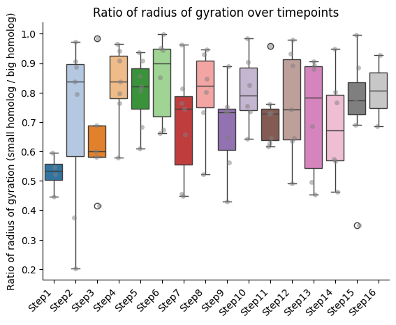
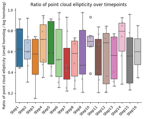
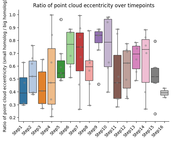
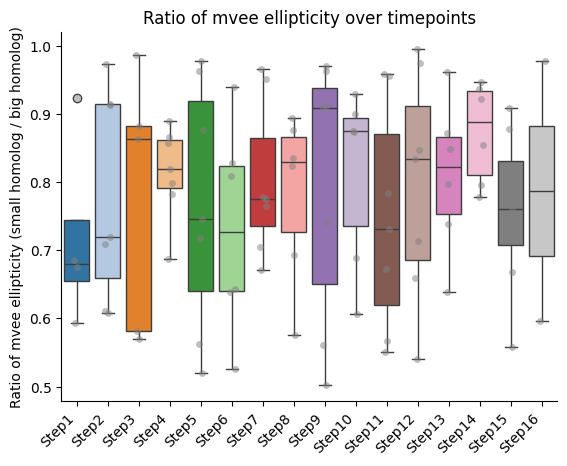
Barplots for the different features across the different timepoints
Barplots of the ratios between homologs, seaparated bt chromatin segment
if both_homs_detected > 0:
    for ratio_name in ratios2calculate:

        temp = ratio_df[["timepoint", ratio_name, "name"]].copy()

        temp["name"] = pd.Categorical(temp["name"], categories=info_df[info_file_dict["column_name"]].tolist(), ordered=True)
        temp.sort_values("name", inplace=True)

        sns.boxplot(data=temp, x="timepoint", y=ratio_name, hue="timepoint", palette="tab20", legend=False)
        sns.stripplot(data=temp, x="timepoint", y=ratio_name, color="gray", dodge=True, alpha=0.5)
        plt.xticks(ticks = range(len(temp["name"].unique())), labels=temp["name"].unique(),
                rotation=45, ha="right")
        plt.xlabel("")
        plt.ylabel(f"Ratio of {' '.join(ratio_name.split('_'))} (small homolog / big homolog)")
        sns.despine()
        plt.title(f"Ratio of {' '.join(ratio_name.split('_'))} over timepoints")
        if save_plots:
            filename = f'boxplot_ratio_{ratio_name.replace(" ", "_")}_homologs' + (f"_{file_suffix}" if file_suffix != '' else '') + '.pdf'
            plot_filename = Path(plots_folder, filename)
            print(f"Saving plots to: {plot_filename}")
            plt.savefig(plot_filename, **plot_opts)
            del filename, plot_filename
        else:
            plt.show()
        plt.close()

    # del ratio_name, ratios2calculate
# del both_homs_detected, ratio_df