4 - Distance extraction

Description: This notebook contains an example on how to read SRX localization data (in csv format) and extract spatial features like center of mass distances bwetween different chromating segments.

The following index has links to the different sections of the notebook. Some sections may have additional indexes to access the subparts.
If you are using VS Code to visualize the notebook, the links may not work. This is due to how VC Code render the notebook. To navigate the notebook use the outline panel. To know more about it, check this link.

Content:

• Library imports

• Setting some variables

• Exporting the data with CIMA

• Spatial features intra-walk

Next notebook to run:
Comparison with orthogonal methods

Library imports and functions

Back to the general index

import re
from pathlib import Path
from collections import defaultdict

import numpy as np
import matplotlib.pyplot as plt
import matplotlib.gridspec as gridspec
from matplotlib.colors import LinearSegmentedColormap
from matplotlib import colormaps
import seaborn as sns
import pandas as pd
from scipy.cluster.hierarchy import linkage
from scipy.spatial.distance import squareform

from cima.parsers.parser_csv import CSVParser
from cima.utils.walk_features import getSpatialFeaturesIntraWalk, convertToMatrix
from cima.utils.misc import calculate_rmsd_matrix, get_dtype_dict

# Set the maximum number of rows to display in the output
pd.options.display.max_rows = 999

# Set the options for saving the plots
plot_opts = {"dpi": 300, "bbox_inches": 'tight', "transparent": True}

# Labels for the plots of the features, so they look nice
plot_labels={
    "volume":"Volume ($nm^3$)",
    "area":"Area ($nm^2$)",
    "sphericity":"Sphericity",
    "sphericity_bribiesca":"Sphericity Bribiesca",
    "density_kb":"Density (blink/bp)",
    "density":"Density (blink/$nm^3$)",
    "compaction":"Genomic compactness (bp/$nm^3$)",
    "solidity":"Solidity",
    "radius_of_gyration":"Radius of gyration",
    "point_cloud_ellipticity":"Ellipticity"
    }

# When showing dataframes we want that this are the first columns, so the user can manually search for them (not recomended)
first_cols = ["experimentID", "nucleusID", "chromosome", "homolog", "timepoint", "name", "flag"]

## Regular expressions to get the metadata from the filename
regex_patterns = {
    "nucleusID": re.compile(r"(?i)nuc(\d+)"), # This searches for "Nuc" or "nuc" followed by digits
    "cellID": re.compile(r"(?i)cell(\d+)"), # This searches for "Cell" or "cell" followed by digits
    "locationID" : re.compile(r"(?i)loc-?(\d+)"), # This searches for "Loc" or "loc" followed by optional hyphen and digits
    "date" : re.compile(r"(\d{4}[-\.]\d{2}[-\.]\d{2})"), # This searches for dates in the format YYYY-MM-DD or YYYY.MM.DD
    "homolog" : re.compile(r"_([ABPM01pm])"), ## Added just in case the homolog is in the filename.
    "chromosome" : re.compile(r"(?i)(chr[\d+MXY])") ## Added just in case the chromosome is in the filename.
    }

# Dictionary to change all the data types of the columns of the different dataframes, so the notebook is mor memory
# efficient.
dtype_dict = {
    "experimentID" : "string", "nucleusID" : "string", "chromosome" : "string",
    "homolog" : "string", "timepoint" : np.int16, "Name" :  "string", "flag" : "string", "segment1" : np.int16,
    "segment1_timepoint" : np.int16, "segment2_name" : "string", "flag_seg1" : "string", "segment2" : np.int16,
    "segment2_timepoint" : np.int16, "segment2_name" : "string", "flag_seg2" : "string", "coms_distance" : np.float32,
    "surface_distance" : np.float32, "entanglement" : np.float32, "volume" : np.float32,
    "area" : np.float32, "sphericity_bribiesca" : np.float32, "sphericity" : np.float32, "radius_of_gyration" : np.float32,
    "point_cloud_ellipticity" : np.float32, "point_cloud_eccentricity" : np.float32, "mvee_ellipticity" : np.float32,
    "mvee_eccentricity" : np.float32, "solidity" : np.float32, "holeless_solidity" : np.float32,
    "numerosity" : np.uint32, "compaction" : np.float32, "density" : np.float32, "density_kb" : np.float32
}

# We create a color map that goes from white to red for the HiC plots (put it in CIMA)
if "bright_red" not in colormaps:
    colormaps.register(name="bright_red", cmap=LinearSegmentedColormap.from_list("bright_red", [(1,1,1),(1,0,0)]))

# Function to plot mean vs variance heatmap of a given feature
def mean_vs_variance_heatmap(mean_matrix, std_matrix, nice_name, timepoint_name_dict, hm_color = "Reds_r"):

    """
    Plot the heatmaps corresponding to the mean and std matrices for a given feature.

    Parameters
    ----------
    mean_matrix : np.ndarray
        2D array representing the mean values.
    std_matrix : np.ndarray
        2D array representing the standard deviation values.
    nice_name : str
        Nice name of the feature to be displayed in the plot titles and colorbars.
    timepoint_name_dict : dict
        Dictionary mapping timepoint indices to their names for labeling axes.
    hm_color : str, optional
        Color map to use for the mean heatmap (default is "Reds_r").
    
    Returns
    -------
    None
    """

    _, ax = plt.subplots(nrows = 1, ncols =2, figsize=(13,5))

    sns.heatmap(
        data = mean_matrix, 
        ax = ax[0],
        cmap = hm_color,
        square = True,
        vmax = np.nanquantile(mean_matrix, 0.9),
        cbar_kws = {"shrink" : 0.9, "label" : f"Mean {nice_name}"},
        xticklabels = list(timepoint_name_dict.values()),
        yticklabels = list(timepoint_name_dict.values()),
        )
    ax[0].set_xticklabels(ax[0].get_xticklabels(), rotation = 45, ha= "right")
    ax[0].set_title(f"Mean of {nice_name}", fontsize = 14)

    sns.heatmap(
        data = std_matrix,
        ax=ax[1],
        cmap='Blues_r',
        square=True,
        vmax=np.nanquantile(std_matrix, 0.9),
        cbar_kws = {"shrink" : 0.9, "label" : f"Mean {nice_name}"},
        xticklabels = list(timepoint_name_dict.values()),
        yticklabels = list(timepoint_name_dict.values()),
        )
    ax[1].set_xticklabels(ax[1].get_xticklabels(), rotation = 45, ha= "right")
    ax[1].set_title(f"Variation of {nice_name}", fontsize = 14)

    if save_plots:
        filename = f'mean_vs_variance_heatmap_{nice_name.replace(" ", "_")}' + (f"_{file_suffix}" if file_suffix != '' else '') + '.pdf'
        plot_filename = Path(plots_folder, filename)
        print(f"Saving plots to: {plot_filename}")
        plt.savefig(plot_filename, **plot_opts)
    else:
        plt.show()

    plt.close()

Setting some variables

In the following cell you should set up some variables for the script to run properly. Change the variables at your convenience, and then you can press “Run all” in the Jupyter Notebook.

Brief explanation of the different variables:

• work_folder: this variable is where the plots and the tsv files that the script creates will be stored.

• data_file: this variable is where the csv files to be assessed are stored.

• info_file: file that contains information about your walks, such as the chromosome, start and end of the steps. You need a columns that matches the ‘timepoint’ column in the csv files, to be able to show proper information.

• column_round: the column that matches the ‘timepoint’ column in the csv files.

• column_name: the column with the “nice” name for the steps. This will be used instead of the timepoint number. Use “” in case the information file does not have this column (in this case the name of the steps will be in the form of ‘StepN’ where N is an incremental number form 1 to the max number of steps).

• column_size: the column for the size of the segment. Use “” in case the information file does not have this column (in this case the notebook will calculate the size automatically of the segments according to the start and end positions in the file).

• column_start_pos: the column of the start position of the timepoint.

• column_end_pos: the column of the start position of the timepoint.

• number_of_steps_library: the number of steps in your library.

• starting_step: the step at which analysis should start.

• prec_mean_dataset: the worst precision of the three axes (usually the Z). This will be used as a blurring factor when creating the 3D maps to calculate the volumetric features.

• save_plots: save the plots into a folder or show them in the notebook.

• file_suffix: add a suffix to the different files created, in case you wish to save the results from different assessments in the same folder. It will be added as “_suffix” before the .tsv/.pdf

The notebook will create a folder in the work_folder path called 4_distance_extraction. Inside this folder 2 subfolders will be created, one for tsvs and one for plots. Inside each folder, a sub-subfolder with the suffix name will have the plots/tsvs for that experiment.

4_distance_extraction/
|-- tsvs/
|   |-- example_tsv_SUFFIX.tsv
|-- plots/
|   |-- example_plot_SUFFIX.pdf

Back to the general index

work_folder = "/scratch/CIMA_tutorial/"
data_folder = "/scratch/CIMA_tutorial/data/chr3"

info_file = "/scratch/CIMA_tutorial/data/chr3/Info_chr3.txt"

column_round = "Round"
column_name = "Name"
column_size = "Size(kb)"
column_chr = "Chr"
column_start_pos = "Start(hg19)"
column_end_pos = "End(hg19)"

number_of_steps_library = 16
starting_step = 6

prec_mean_dataset = 30

save_plots = False

file_suffix = "chr3"

work_folder = Path(work_folder)
data_folder = Path(data_folder)
pre_assessment_folder = Path(work_folder, "2_experimental_quality_assessment")
reconstruction_tsv_folder = Path(work_folder, "3_3D_reconstruction_assessment", "tsvs", file_suffix)

info_df = pd.read_table(Path(info_file), sep="\t")
info_df.columns = info_df.columns.str.strip() # In case there are leading or trailing spaces in the column names

info_file_dict = {
    "column_round" : column_round,
    "column_name" : column_name,
    "column_size" : column_size,
    "column_chr" : column_chr,
    "column_start_pos" : column_start_pos,
    "column_end_pos" : column_end_pos,
}

del column_round, column_name, column_size, column_chr, column_start_pos, column_end_pos, info_file

Exporting the data with CIMA

Content:

• Creating the list of CIMA StructuralObject

• Checking the information file

• Creating a color palette and the results folders

Back to the general index

Creating the list of CIMA StructuralObjects

In this cell we create a list of StructuralObjects (the main CIMA class type).
This list is the basis to do the assessment through this Jupyter Notebook.

When loading the data, we will also take out those traces or CS that did not pass the assessment in the previous notebooks.

When reading the file, it will also add some metadata gathered from the filename of the csv file:

• nucleusID: searches for "nuc" (with any combination of lower and upper case) followed by digits. If there is not a match, the default is filecount (first file read will be number 1, ...).


• cellID: searches for "cell" (with any combination of lower and upper case) followed by digits. If there is not a match, the default is filecount (first file read will be number 1, ...).


• locationID: searches for "loc" (with any combination of lower and upper case) followed by optional hyphen and digits.If there is not a match, the default is filecount (first file read will be number 1, ...).


• date: searches for dates in the format YYYY-MM-DD or YYYY.MM.DD. If there is not a match, the default is the file name.


• homolog: searches for "_" followed by A, B, M, P, m, p, 0 or 1 (only one instance of this). If there is not a match, the default is "A".


• chromosome: searches for "chr" (with any combination of lower and upper case) followed by a number, M, X or Y. If there is not a match, the default is "chrN".

Back to the section index

# Get a list of all CSV files in the specified data folder
csv_files = list(data_folder.glob('*.csv'))

if len(csv_files) == 0:
    print("No files found, please input the correct work_folder")
else:
    print(f"Total number of files found: {len(csv_files)}")

print("Loading the experimental quality data from the CSV files")
traces_pass = pd.read_csv(Path(pre_assessment_folder, f"experimental_assessment_pass_{file_suffix}.txt"), sep="\t", names=["trace"])

print("Loading the bad flags from the CSV files")
segments_to_remove_CCC = pd.read_csv(Path(reconstruction_tsv_folder, f'segments2remove_bycccvariation_t2{("_" + file_suffix) if file_suffix != "" else ""}.tsv'), sep="\t")
if "flag" not in segments_to_remove_CCC.columns and not segments_to_remove_CCC.empty:
    print("\tCreating the 'flag' column for reconstruction-based removal")
    segments_to_remove_CCC["flag"] = segments_to_remove_CCC[["experimentID", "nucleusID", "homolog", "timepoint"]].astype(str).apply("_".join, axis=1)
    bad_flags = set(segments_to_remove_CCC["flag"].astype(str).values)
elif not segments_to_remove_CCC.empty:
    bad_flags = set(segments_to_remove_CCC["flag"].astype(str).values)
else:
    bad_flags = set()

# Get a list of metadata keys to extract from filenames
metadata_keys = ["nucleusID", "cellID", "locationID", "date", "homolog", "chromosome"]

# Initialize an empty list to store the StructuralObject instances
obj_list = []

if len(csv_files) > 0:
    # Iterate over each file in the list of file names
    for count, filein in enumerate(csv_files, start=1):

        stem = Path(filein).stem

        if not stem in traces_pass["trace"].values:
            print(f"Skipping file {count}: {stem} because it did not pass the experimental quality assessment.")
            continue

        print(f"Processing file {count}: {stem}", end="\r")

        # We mine the metadata from the filename using regex patterns. If not possible, assign default values.
        # In the case of nucleus, cell and location, the default is the filecount (first file read will be number 1, ...)
        # In the case of date, if no date can be found, the filename gets used.
        # If no valid homolog denomination is found, the default value is A.
        # If no valid chromosome denomination is found, the default value is chrN.
        metadata_CIMA = {
            key: (match.group(1) if (match := regex_patterns[key].search(stem)) else default)
            for key, default in zip(metadata_keys, [count, count, count, stem, "A", "chrN"])
        }

        # Adjust the metadata for nucleus and cell (if nucleus is count, but cell is something, use the cell match in nucleus)
        if "cellID" in metadata_CIMA and metadata_CIMA["nucleusID"] == count:
            metadata_CIMA["nucleusID"] = metadata_CIMA["cellID"]

        # Set experimentID as date for consistency
        metadata_CIMA["experimentID"] = metadata_CIMA["date"]

        # Read the CSV file and create a StructuralObject instance
        objin = CSVParser.read_CSV_file(filein.as_posix(), metadata = metadata_CIMA, content_type = "srx")

        # Filter the atomList to include only the specified timepoints in the info file
        objin.atomList = objin.atomList[(objin.atomList['timepoint'] >= starting_step - 1) &
                                        (objin.atomList['timepoint'] < (starting_step + number_of_steps_library - 1))].copy()
        
        experiment_id = objin.metadata["experimentID"]
        nucleus_id = int(objin.metadata["nucleusID"])
        homolog = objin.metadata["homolog"]
        
        full_flags = (experiment_id + "_" + str(nucleus_id) + "_" +homolog + "_" + objin.atomList["timepoint"].astype(str))
        remove_mask = full_flags.isin(bad_flags)

        if remove_mask.any():
            removed_tps = objin.atomList.loc[remove_mask, "timepoint"].unique()
            # removed_tps = ",".join([tp_names[tp] for tp in removed_tps])
            # print(f"Excluding timepoints {removed_tps} in experimentID: {experiment_id}, nucleusID: {nucleus_id}, homolog: {homolog} due to poor assessment.")
            objin.atomList = objin.atomList.loc[~remove_mask].copy()

        for tp in objin.atomList["timepoint"].unique():
            # Take out the timepoint from the atomList if it has less tha 10 points
            tp_mask = objin.atomList["timepoint"] == tp
            if tp_mask.sum() < 10:
                print(f"\tExcluding timepoint {tp} in experimentID: {experiment_id}, nucleusID: {nucleus_id}, homolog: {homolog} because it has less than 10 points.")
                objin.atomList = objin.atomList.loc[~tp_mask].copy()
        
        # Append the object to the list
        obj_list.append(objin)

    # Nice print to tell the user the number of objects created.
    print(f"\nTotal number of objects created: {len(obj_list)}")

    # Clean up memory by deleting some of the variables no longer needed
    del count, filein, stem, metadata_CIMA, match, objin

del csv_files, metadata_keys
del bad_flags
del experiment_id, nucleus_id, homolog, full_flags, remove_mask
if 'segments_to_remove_precision' in locals():
    del segments_to_remove_CCC

Total number of files found: 33
Loading the experimental quality data from the CSV files
Loading the bad flags from the CSV files
	Creating the 'flag' column for reconstruction-based removal
Skipping file 2: 2018-07-10_nuc04_A_chr3 because it did not pass the experimental quality assessment.
Skipping file 5: 2018-07-10_nuc03_A_chr3 because it did not pass the experimental quality assessment.
	Excluding timepoint 19 in experimentID: 2018-09-04, nucleusID: 7, homolog: A because it has less than 10 points.
Skipping file 26: 2018-09-04_nuc01_A_chr3 because it did not pass the experimental quality assessment.
Processing file 33: 2018-09-04_nuc06_A_chr3
Total number of objects created: 30

Checking the information file

This cells makes an adjustment in the info_df.

It checks if the column of the info_df that we will use as the link between this data frame and our walks has the same timepoints. This happens because most programs start with timepoint 0, while most information files start at timepoint 1.

This will create a new column in the dataframe that is called ‘timepoint’. This column will be modified so it has the same range as the timepoint column from the csv files.

Back to the section index

list_of_timepoints = sorted({int(tp) for obj in obj_list for tp in obj.atomList.timepoint.unique()})
info_of_timepoints = list(map(int, info_df[info_file_dict["column_round"]].tolist()))

print(f'List of timepoints found across all objects: {list_of_timepoints}')
print(f'List of timepoints in the information file: {info_of_timepoints}\n')

if list_of_timepoints == info_of_timepoints:
    print('The timepoints found in the objects match those in the information file.')
    info_df["timepoint"] = info_df[info_file_dict["column_round"]]
elif set(list_of_timepoints).issubset(info_of_timepoints):
    print('Note: The timepoints found in the objects are a subset of those in the information file. Not all timepoints are present.')
    info_df["timepoint"] = info_df[info_file_dict["column_round"]]
elif list_of_timepoints == [x - 1 for x in info_of_timepoints]:
    print('Note: The column for the information file that has the timepoint is offset by 1 compared to the objects, adjusting accordingly.')
    info_df["timepoint"] = info_df[info_file_dict["column_round"]] - 1
elif set(list_of_timepoints).issubset({x - 1 for x in info_of_timepoints}):
    print('Note: The timepoints found in the objects are a subset of those in the information file, which are offset by 1 compared to the objects. Adjusting accordingly.')
    info_df["timepoint"] = info_df[info_file_dict["column_round"]] - 1
else:
    print('Warning: The timepoints found in the objects do not match those in the information file.')

if info_file_dict["column_size"] == "":
    print("Calculating size column from start and end positions...")
    column_size = "size"
    info_file_dict["column_size"] = column_size
    info_df[column_size] = info_df[info_file_dict["column_end_pos"]] - info_df[info_file_dict["column_start_pos"]]

if info_file_dict["column_name"] == "":
    print("Setting name column from round numbers...")
    info_file_dict["column_name"] = "name"
    info_df["name"] = [f"Step{i}" for i in range(1, info_df.shape[0]+1)]

tp_names = info_df.set_index("timepoint")[info_file_dict["column_name"]].to_dict()
    
del list_of_timepoints, info_of_timepoints

List of timepoints found across all objects: [5, 6, 7, 8, 9, 10, 11, 12, 13, 14, 15, 16, 17, 18, 19, 20]
List of timepoints in the information file: [6, 7, 8, 9, 10, 11, 12, 13, 14, 15, 16, 17, 18, 19, 20, 21]

Note: The column for the information file that has the timepoint is offset by 1 compared to the objects, adjusting accordingly.

Creating a color palette and the results folders for the tsv and plot files

Here we create a color palette automatically based on the different experiment ID found across the files. Experiment IDs are usually the date of the experiment. This allows to easily check for a possible batch effect.

We also create the folders were to store the results.

• 4_distance_extraction/tsvs: a subfolder using the suffix name will be created, where the different tsv files will be stored.


• 4_distance_extraction/plots: a subfolder using the suffix name will be created, where the different plots (in pdf format) will be stored.

Back to the section index

# Define the color palette for experiments. Use the date or the experimentID (date) as the key.
color_palette = {exp_date: color for exp_date, color in zip(
    # We get a set of unique dates from the metadata of the objects
    set([file.metadata["experimentID"] for file in obj_list]),
    # We assign a color from the tab10 palette for each unique date
    sns.color_palette("tab10", n_colors=len(set([file.metadata["experimentID"] for file in obj_list]))) 
)}

# This palette is fixed for the current experiments used in the tutorial, which aim to reproduce the figures in the CIMA paper.
color_palette = {'2018-01-11':"#a6cee3" ,'2018-06-28':'#1f78b4', '2018-07-10':'#b2df8a', '2018-09-04':'#33a02c'}

# Create the folders to save the results. If the folders already exist, do not raise an error.
tsv_folder = Path(work_folder, "4_distance_extraction", "tsvs", file_suffix)
tsv_folder.mkdir(parents=True, exist_ok=True)

plots_folder = Path(work_folder, "4_distance_extraction", "plots", file_suffix)
plots_folder.mkdir(parents=True, exist_ok=True)

Spatial feature intra-walk

Content:

• Spatial feautre intra-walk calculation

• Boxenplots for the different distances calculated

• Mean, variation and RMSD matrices calculation for the different distances

• Plot the variation matrices for the different distances

Back to the general index

Spatial feature intra-walk calculations

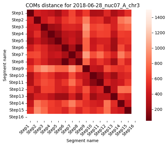
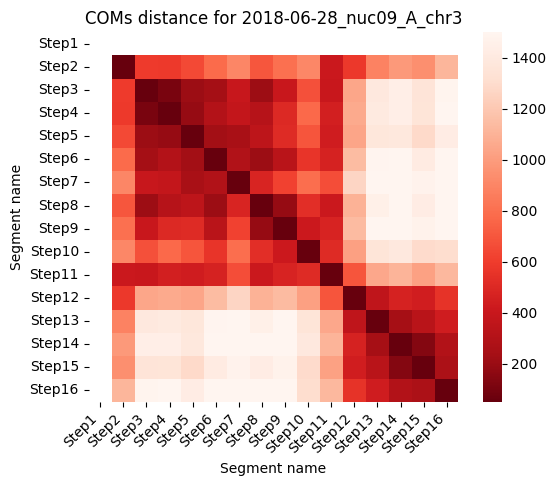
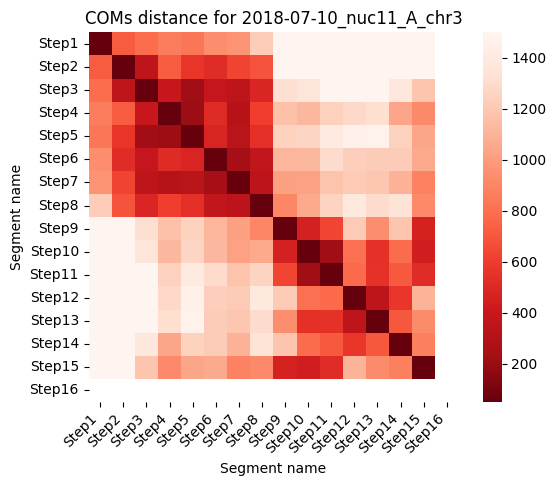
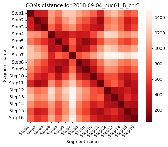
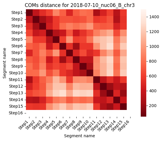
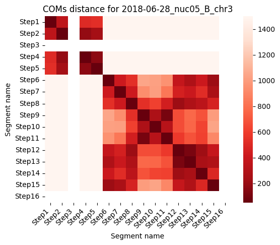
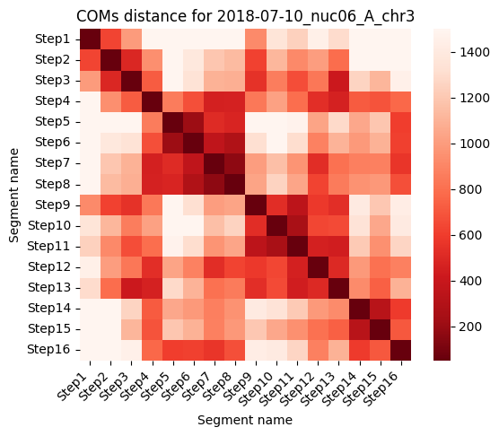
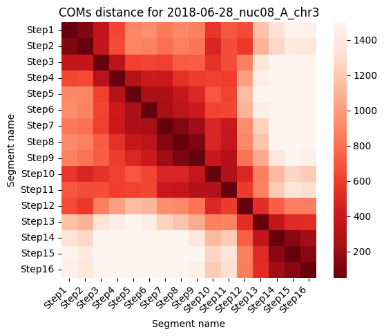
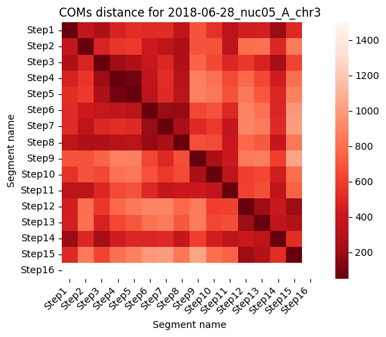
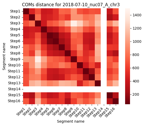
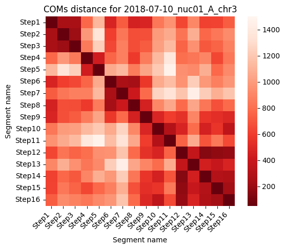
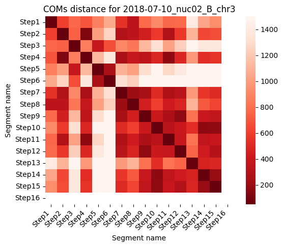
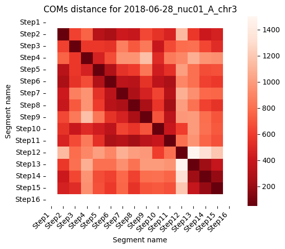
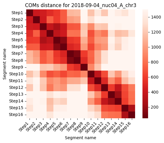
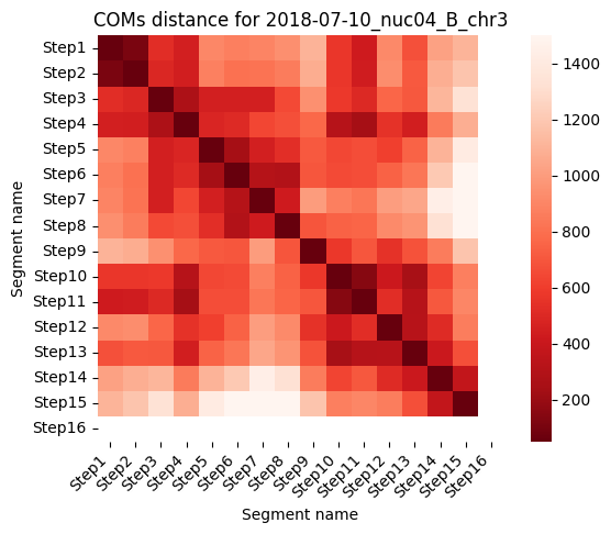
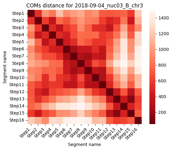
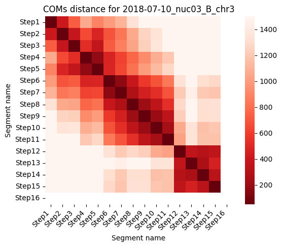
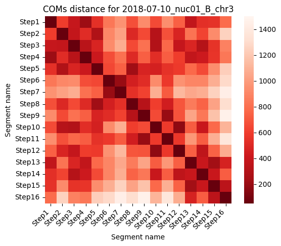
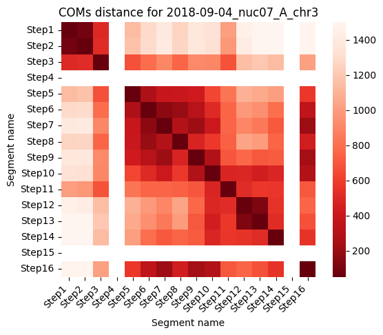
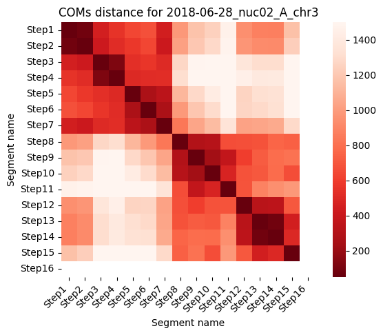
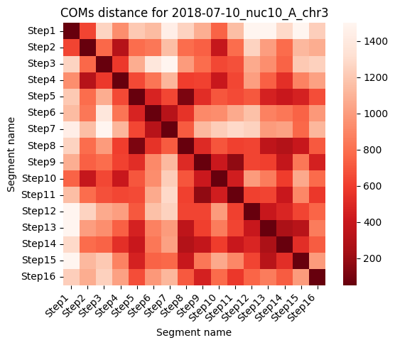
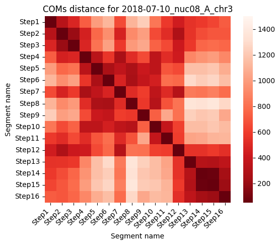
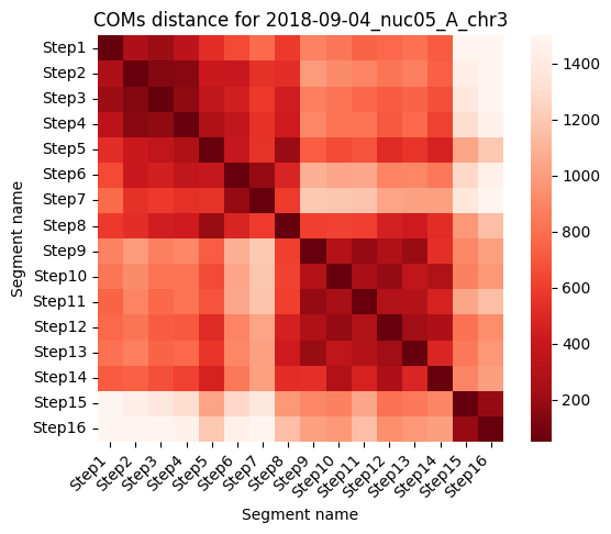
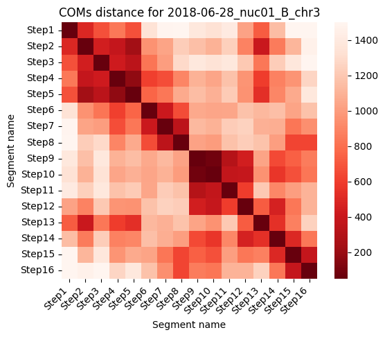
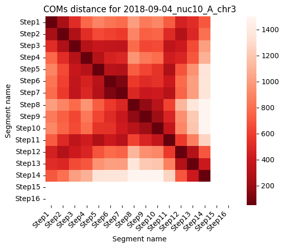
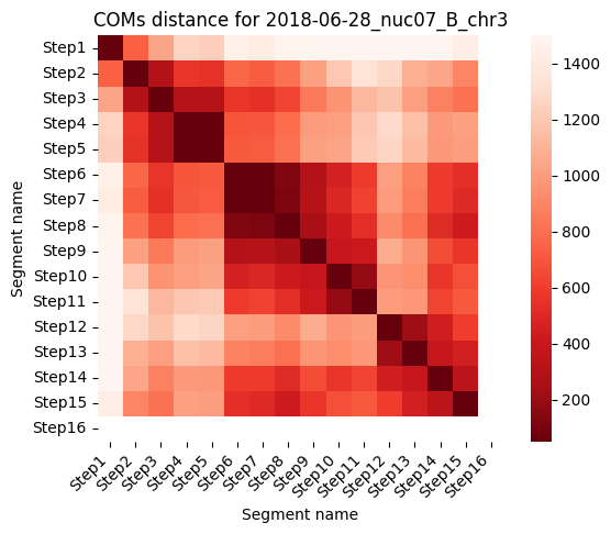
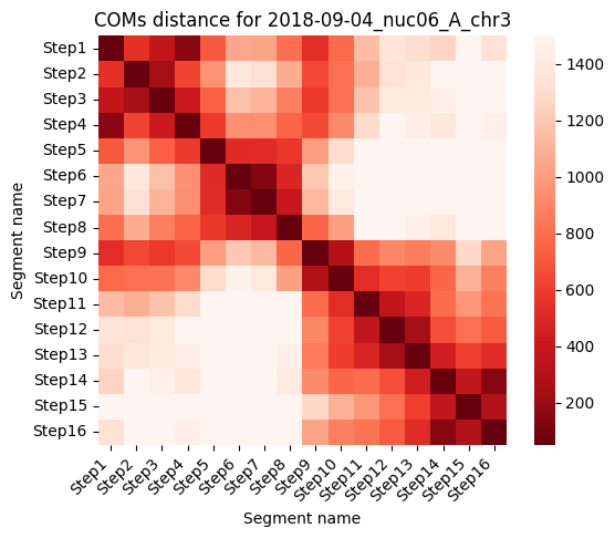
Here we will calculate the COM distance, surface distance and entanglement for every pair of segments for every walk.

If this has already been calculated and saved into a file called “spatial_features_SUFFIX.tsv”, the file will be loaded.

If the file is not located, then the notebook will perform the calculations and store that data in the file.

Back to the section index

last_cols = ["segment1", "segment1_timepoint", "segment1_name", "flag_seg1", 
             "segment2", "segment2_timepoint", "segment2_name", "flag_seg2", 
             "coms_distance", "surface_distance", "entanglement"]

spatial_tsv_filename = f"spatial_features_{prec_mean_dataset}{('_' + file_suffix if file_suffix != '' else '')}.tsv"

try:
    print("Trying to read pre-calculated spatial features by pairs from TSV file...")
    dataframe_spatialfeatures = pd.read_csv(Path(tsv_folder, spatial_tsv_filename), sep='\t')
    dataframe_spatialfeatures["flag"] = dataframe_spatialfeatures[["experimentID","nucleusID","homolog"]].astype(str).apply('_'.join, axis=1)
    dataframe_spatialfeatures["flag_seg1"] = dataframe_spatialfeatures[["experimentID","nucleusID","homolog","segment1_timepoint"]].astype(str).apply('_'.join, axis=1)
    dataframe_spatialfeatures["flag_seg2"] = dataframe_spatialfeatures[["experimentID","nucleusID","homolog","segment2_timepoint"]].astype(str).apply('_'.join, axis=1)

    print("Pre-calculated spatial features by pairs loaded from TSV file.")

except FileNotFoundError:
    print("Pre-calculated TSV file not found. Calculating spatial features by pairs from scratch...")

    df_list=[]

    for file_counter, obj_in in enumerate(obj_list, start = 1):

        print(f"Processing contact matrix for file {file_counter}/{len(obj_list)}: {Path(obj_in.metadata['filename']).stem}")

        list_CS=obj_in.split_into_time(return_list = True)

        temp_df = getSpatialFeaturesIntraWalk(list_CS, prec_mean = prec_mean_dataset, n_jobs = 8, verbose = False)
        
        temp_df["segment1_name"] = [tp_names[tp] for tp in temp_df["segment1_timepoint"]]
        temp_df["segment2_name"] = [tp_names[tp] for tp in temp_df["segment2_timepoint"]]
        temp_df["experimentID"] = obj_in.metadata["experimentID"]
        temp_df["nucleusID"] = obj_in.metadata["nucleusID"]
        temp_df["homolog"] = obj_in.metadata["homolog"]
        temp_df["chromosome"] = obj_in.metadata["chromosome"]
        
        temp_df["flag"] = temp_df[["experimentID","nucleusID","homolog"]].astype(str).apply('_'.join, axis=1)
        temp_df["flag_seg1"] = temp_df[["experimentID","nucleusID","homolog","segment1_timepoint"]].astype(str).apply('_'.join, axis=1)
        temp_df["flag_seg2"] = temp_df[["experimentID","nucleusID","homolog","segment2_timepoint"]].astype(str).apply('_'.join, axis=1)

        df_list.append(temp_df)

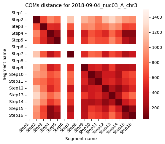
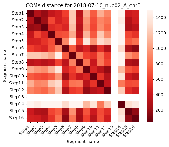
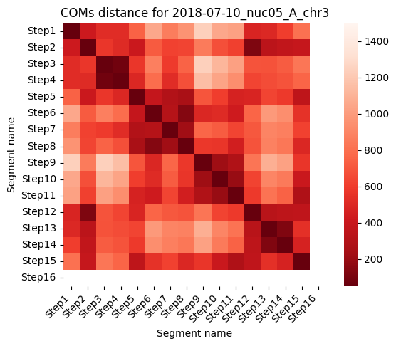
        mat = convertToMatrix(pairs_features_df = temp_df,
                              value = "coms_distance",
                              cluss = np.array(info_df.timepoint.tolist()))

        mat = mat.astype(np.float64)

        x_labels = info_df.set_index("timepoint").loc[mat.index.tolist()]["Name"].tolist()
        y_labels = info_df.set_index("timepoint").loc[mat.columns.tolist()]["Name"].tolist()

        sns.heatmap(mat, cmap='Reds_r', square=True,
                    vmin=50.,vmax=1500,
                    xticklabels=x_labels,
                    yticklabels=y_labels)
        
        plt.xlabel("Segment name")
        plt.xticks(rotation=45, ha='right')
        plt.ylabel("Segment name")
        plt.title(f"COMs distance for {Path(obj_in.metadata['filename']).stem}")
        if save_plots:
            filename = f'com_distance_{prec_mean_dataset}_{Path(obj_in.metadata["filename"]).stem}' + (f"_{file_suffix}" if file_suffix != '' else '') + '.pdf'
            plot_filename = Path(plots_folder, filename)
            print(f"\tSaving plots to: {plot_filename}")
            plt.savefig(plot_filename, **plot_opts)
            del filename, plot_filename
        else:
            plt.show()
        plt.close()

    # Concatenate all the dataframes.
    dataframe_spatialfeatures = pd.concat(df_list, ignore_index=True)

    # Reorder the columns, so the table looks nicer and it is easier to manually search for entries.
    cols = dataframe_spatialfeatures.columns.tolist()
    cols_reorder = [col for col in first_cols if col in cols] + last_cols
    dataframe_spatialfeatures = dataframe_spatialfeatures[cols_reorder]

    print("Calculating spatial features by pairs... Done!")

    # Save the dataframe to a TSV file
    print(f"Saving spatial features by pairs to TSV file: {spatial_tsv_filename}...", end="\r")
    dataframe_spatialfeatures.drop(columns=["flag", "flag_seg1","flag_seg2"]).to_csv(Path(tsv_folder, spatial_tsv_filename), sep='\t', index=None)
    print(f"Saving spatial features by pairs to TSV file: {spatial_tsv_filename}... Done!")

    del file_counter, obj_in, list_CS, temp_df, mat, x_labels, y_labels, df_list, cols, cols_reorder

# Define the desired dtypes for specific columns.
dataframe_spatialfeatures = dataframe_spatialfeatures.astype(get_dtype_dict(dataframe_spatialfeatures.columns.to_list(), dtype_dict))

# Reorder the columns, so the table looks nicer and it is easier to manually search for entries.
cols = dataframe_spatialfeatures.columns.tolist()
cols_reorder = [col for col in first_cols if col in cols] + last_cols
dataframe_spatialfeatures = dataframe_spatialfeatures[cols_reorder]

display(dataframe_spatialfeatures.head())

del last_cols, spatial_tsv_filename, cols, cols_reorder

Trying to read pre-calculated spatial features by pairs from TSV file...
Pre-calculated TSV file not found. Calculating spatial features by pairs from scratch...
Processing contact matrix for file 1/30: 2018-09-04_nuc03_A_chr3

Processing contact matrix for file 2/30: 2018-07-10_nuc02_A_chr3

Processing contact matrix for file 3/30: 2018-07-10_nuc05_A_chr3

Processing contact matrix for file 4/30: 2018-06-28_nuc07_A_chr3

Processing contact matrix for file 5/30: 2018-06-28_nuc09_A_chr3

Processing contact matrix for file 6/30: 2018-07-10_nuc11_A_chr3

Processing contact matrix for file 7/30: 2018-09-04_nuc01_B_chr3

Processing contact matrix for file 8/30: 2018-07-10_nuc06_B_chr3

Processing contact matrix for file 9/30: 2018-06-28_nuc05_B_chr3

Processing contact matrix for file 10/30: 2018-07-10_nuc06_A_chr3

Processing contact matrix for file 11/30: 2018-06-28_nuc08_A_chr3

Processing contact matrix for file 12/30: 2018-06-28_nuc05_A_chr3

Processing contact matrix for file 13/30: 2018-07-10_nuc07_A_chr3

Processing contact matrix for file 14/30: 2018-07-10_nuc01_A_chr3

Processing contact matrix for file 15/30: 2018-07-10_nuc02_B_chr3

Processing contact matrix for file 16/30: 2018-06-28_nuc01_A_chr3

Processing contact matrix for file 17/30: 2018-09-04_nuc04_A_chr3

Processing contact matrix for file 18/30: 2018-07-10_nuc04_B_chr3

Processing contact matrix for file 19/30: 2018-09-04_nuc03_B_chr3

Processing contact matrix for file 20/30: 2018-07-10_nuc03_B_chr3

Processing contact matrix for file 21/30: 2018-07-10_nuc01_B_chr3

Processing contact matrix for file 22/30: 2018-09-04_nuc07_A_chr3

Processing contact matrix for file 23/30: 2018-06-28_nuc02_A_chr3

Processing contact matrix for file 24/30: 2018-07-10_nuc10_A_chr3

Processing contact matrix for file 25/30: 2018-07-10_nuc08_A_chr3

Processing contact matrix for file 26/30: 2018-09-04_nuc05_A_chr3

Processing contact matrix for file 27/30: 2018-06-28_nuc01_B_chr3

Processing contact matrix for file 28/30: 2018-09-04_nuc10_A_chr3

Processing contact matrix for file 29/30: 2018-06-28_nuc07_B_chr3

Processing contact matrix for file 30/30: 2018-09-04_nuc06_A_chr3

Calculating spatial features by pairs... Done!
Saving spatial features by pairs to TSV file: spatial_features_30_chr3.tsv... Done!

	experimentID	nucleusID	chromosome	homolog	flag	segment1	segment1_timepoint	segment1_name	flag_seg1	segment2	segment2_timepoint	segment2_name	flag_seg2	coms_distance	surface_distance	entanglement
0	2018-09-04	03	chr3	A	2018-09-04_03_A	1	6	Step2	2018-09-04_03_A_6.0	1	6	Step2	2018-09-04_03_A_6.0	0.000000	0.000000	1.0
1	2018-09-04	03	chr3	A	2018-09-04_03_A	1	6	Step2	2018-09-04_03_A_6.0	2	7	Step3	2018-09-04_03_A_7.0	648.681274	439.360504	0.0
2	2018-09-04	03	chr3	A	2018-09-04_03_A	1	6	Step2	2018-09-04_03_A_6.0	3	8	Step4	2018-09-04_03_A_8.0	893.308655	634.317383	0.0
3	2018-09-04	03	chr3	A	2018-09-04_03_A	1	6	Step2	2018-09-04_03_A_6.0	4	9	Step5	2018-09-04_03_A_9.0	773.690552	373.377441	0.0
4	2018-09-04	03	chr3	A	2018-09-04_03_A	1	6	Step2	2018-09-04_03_A_6.0	5	11	Step7	2018-09-04_03_A_11.0	1190.255737	982.187744	0.0

Boxenplots for the COMs distance, surface distance and entanglement between the different segments of the same walk

Boxenplots to show the distribution of the different Back to the section index

data_table = defaultdict(list)

for feature in ['coms_distance', 'surface_distance', 'entanglement']:

    nice_name = feature.replace('_', ' ')

    plt.figure(figsize=(4,6))
    sns.boxenplot(y=dataframe_spatialfeatures[feature].astype(float))
    plt.title(f"Distribution of {nice_name} over all segment pairs")
    plt.ylabel(nice_name)
    sns.despine()
    if save_plots:
        filename = f'{feature}_distribution_allsegments_bypairs' + (f"_{file_suffix}" if file_suffix != '' else '') + '.pdf'
        plot_filename = Path(plots_folder, filename)
        print(f"Saving plots to: {plot_filename}")
        plt.savefig(plot_filename, **plot_opts)
        del filename, plot_filename
    else:
        plt.show()
    plt.close()

    data_table["feature"].append(nice_name)
    data_table["min"].append(np.round(dataframe_spatialfeatures[feature].min(), decimals = 4))
    data_table["25% quantile"].append(np.round(dataframe_spatialfeatures[feature].quantile(0.25), decimals = 4))
    data_table["median"].append(np.round(dataframe_spatialfeatures[feature].quantile(0.5), decimals = 4))
    data_table["75% quantile"].append(np.round(dataframe_spatialfeatures[feature].quantile(0.75), decimals = 4))
    data_table["max"].append(np.round(dataframe_spatialfeatures[feature].max(), decimals = 4))

data_table = pd.DataFrame(data_table).set_index("feature").T
display(data_table)

del feature, nice_name, data_table

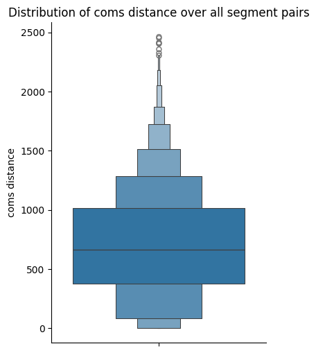
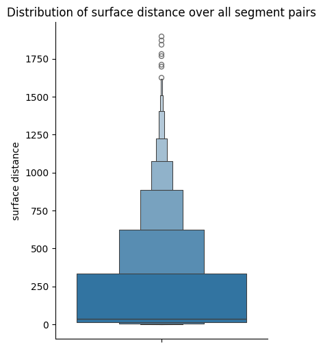
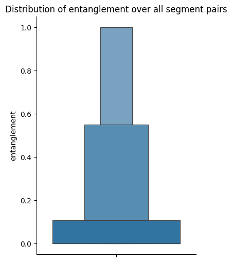
feature	coms distance	surface distance	entanglement
min	0.000000	0.000000	0.0000
25% quantile	373.764300	13.145400	0.0000
median	661.103100	36.201000	0.0000
75% quantile	1012.823200	333.694800	0.1079
max	2462.811279	1896.338623	1.0000

Mean, variation and RMSD matrices calculation

Calculate mean and variation matrix for the ensemble of walks.

The notebook will also calculate the RMSD between the mean matrices.

Back to the section index

mean_combined_mats = {}
std_combined_mats = {}
rmsd_combined_mats = {}
collection_combined_mats = {}

for feat in ['coms_distance', 'surface_distance', 'entanglement']:

    print(f"Working on feature: {feat}...")
    
    combined_ent_mat0=[]
    
    # TODO add the power law scaling things.

    for f in dataframe_spatialfeatures.flag.unique().tolist():

        # print(f"\tProcessing flag: {f}...")

        mat = convertToMatrix(pairs_features_df = dataframe_spatialfeatures[dataframe_spatialfeatures.flag == f],
                              value = feat,
                              cluss = np.array(info_df.timepoint.tolist()))

        mat = mat.astype(np.float64)
        combined_ent_mat0.append(mat)
    
    mean_combined_mats[feat] = np.nanmean(combined_ent_mat0, axis=0)
    std_combined_mats[feat] = np.nanstd(combined_ent_mat0, axis=0)
    collection_combined_mats[feat] = (np.invert(np.isnan(combined_ent_mat0))).sum(axis=0)



    # Take out rows/columns that contain 1 or more NaN values
    mean_combined_mats[feat] = mean_combined_mats[feat][~np.isnan(mean_combined_mats[feat]).any(axis=1)][:, ~np.isnan(mean_combined_mats[feat]).any(axis=0)]
    
    std_combined_mats[feat] = std_combined_mats[feat][~np.isnan(std_combined_mats[feat]).any(axis=1)][:, ~np.isnan(std_combined_mats[feat]).any(axis=0)]
    
    if feat != "entanglement":
        rmsd_combined_mats[feat] = calculate_rmsd_matrix(combined_ent_mat0)

        list_of_flags = np.array(dataframe_spatialfeatures.flag.unique().tolist())[~np.isnan(rmsd_combined_mats[feat]).any(axis = 1)]

        rmsd_combined_mats[feat] = rmsd_combined_mats[feat][~np.isnan(rmsd_combined_mats[feat]).any(axis=1)][:, ~np.isnan(rmsd_combined_mats[feat]).any(axis=0)]
    
        rmsd_combined_mats[feat] = pd.DataFrame(rmsd_combined_mats[feat], index = list_of_flags, columns = list_of_flags)

    print(f"Working on feature: {feat}... Done!")

del feat, combined_ent_mat0, f, mat, list_of_flags

Working on feature: coms_distance...
Working on feature: coms_distance... Done!
Working on feature: surface_distance...
Working on feature: surface_distance... Done!
Working on feature: entanglement...
Working on feature: entanglement... Done!

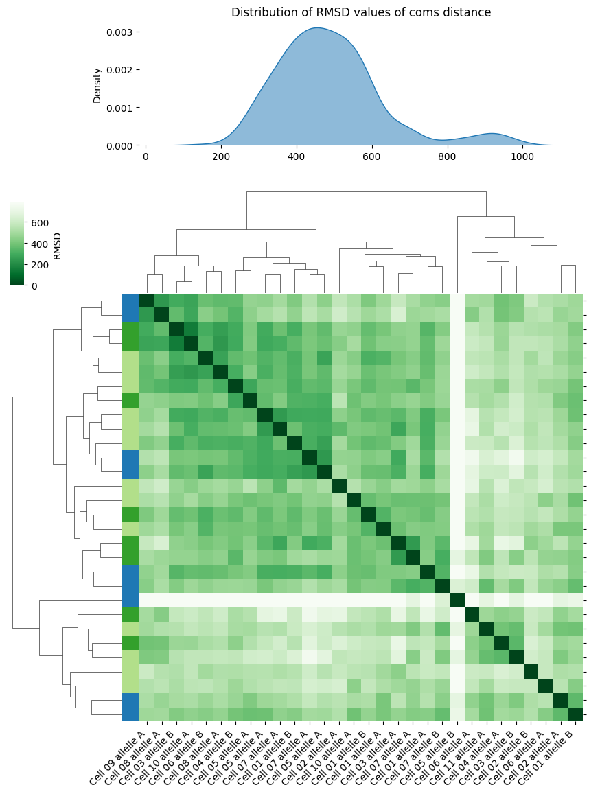
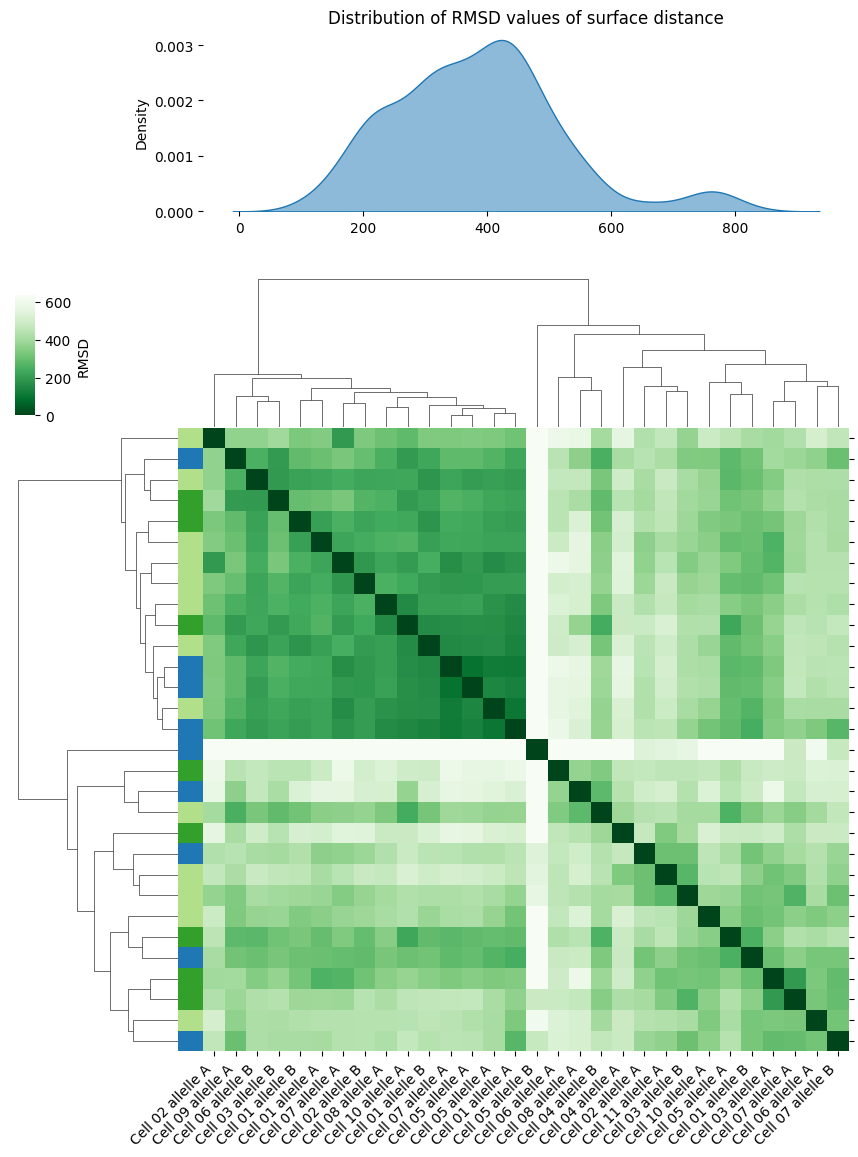
clustermap and density distibution for RMSD values of COM distances and surface distances

# Add eficiency of the file, put it in green

for feature in ["coms_distance", "surface_distance"]:

    print(f"Creating clustermap for feature: {feature}...")
    
    lnk = linkage(squareform(rmsd_combined_mats[feature]), method='ward')

    labels = [f"Cell {n.split('_') [1]} allelle {n.split('_')[2]}" for n in dataframe_spatialfeatures.flag.unique().tolist()]

    g = sns.clustermap(
        data = rmsd_combined_mats[feature], # Matrix of RMSD between the different experiments
        cmap='Greens_r', # Color used 
        xticklabels=labels, # Labels (basically the file where they come from)
        vmax=np.nanquantile(rmsd_combined_mats[feature], 0.95), # Maximum number to do the colors
        row_linkage=lnk, # Pre-calculated linkage for the rows
        col_linkage=lnk, # Pre-calculated linkage for the columns
        row_colors=dataframe_spatialfeatures.groupby("flag").first().experimentID.map(color_palette), # Color the rows by the experiment they come from
        figsize = (10,12)
    )
    
    g.ax_heatmap.set_xticklabels(g.ax_heatmap.get_xticklabels(), rotation=45, ha="right", )
    g.ax_heatmap.set_ylabel("")
    g.ax_heatmap.set_yticklabels([])
    g.ax_row_colors.set_xlabel("")
    g.ax_row_colors.set_xticks([])

    g.gs.update(bottom = 0.05, top = 0.7)

    g.cax.set_position((0.02, 0.58, 0.02, 0.1))
    g.cax.set_ylabel("RMSD", rotation=90, labelpad=4)

    gs2 = gridspec.GridSpec(1, 1, bottom = 0.785)
    ax2 = g.fig.add_subplot(gs2[0])
    ax2.set_position((g.ax_heatmap.get_position().x0, 0.75,
                      g.ax_heatmap.get_position().width, 0.15))
    
    sns.kdeplot(data=rmsd_combined_mats[feature].replace(0, np.nan).to_numpy().flatten(), fill=True, alpha = 0.5, ax=ax2)
    ax2.set_title(f"Distribution of RMSD values of {feature.replace('_', ' ')}")
    sns.despine(top = True, right = True, bottom = True, left = True)

    if save_plots:
        filename = f'{feature}_rmsd_clustermap' + (f"_{file_suffix}" if file_suffix != '' else '') + '.pdf'
        plot_filename = Path(plots_folder, filename)
        print(f"Saving plots to: {plot_filename}")
        plt.savefig(plot_filename, **plot_opts)
        del filename, plot_filename
    else:
        plt.show()

    plt.close()
    
del feature, lnk, g, gs2, ax2, labels

Creating clustermap for feature: coms_distance...

Creating clustermap for feature: surface_distance...

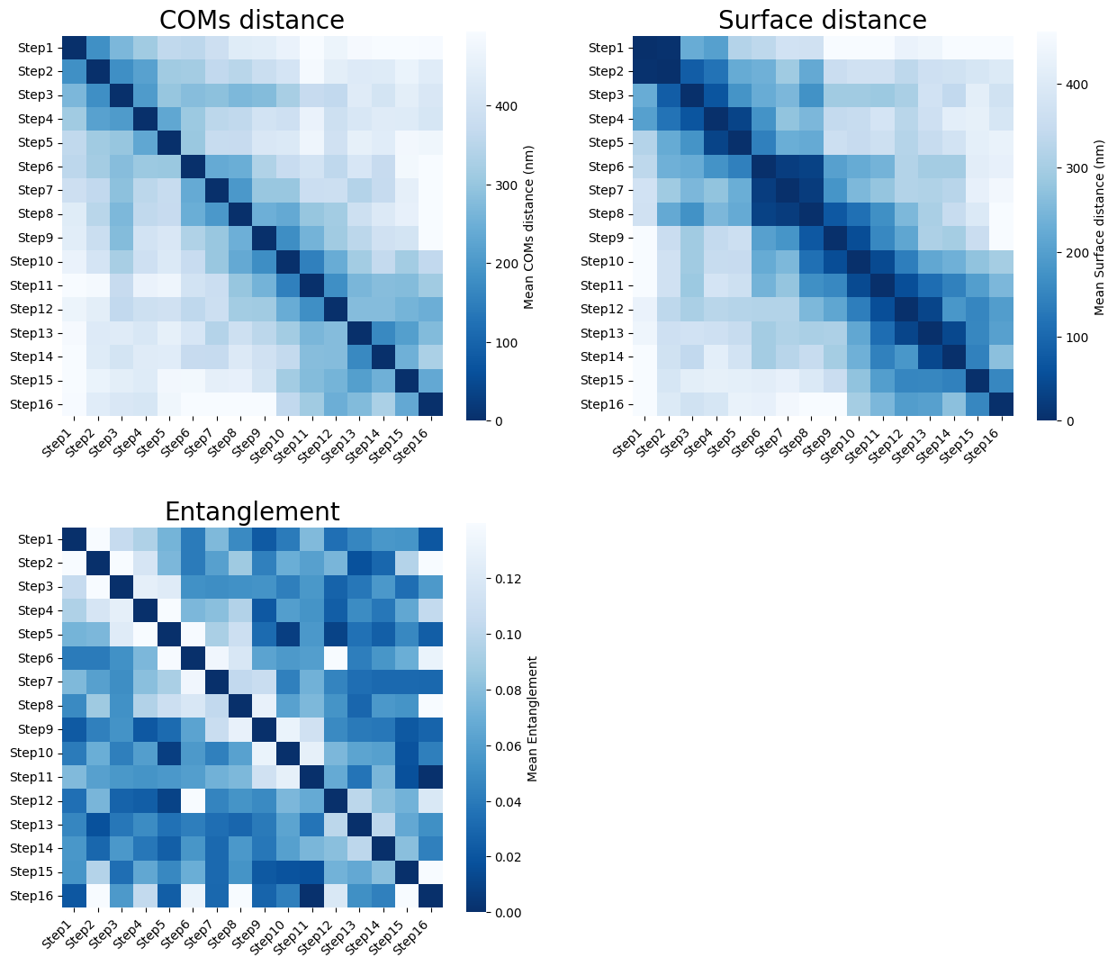
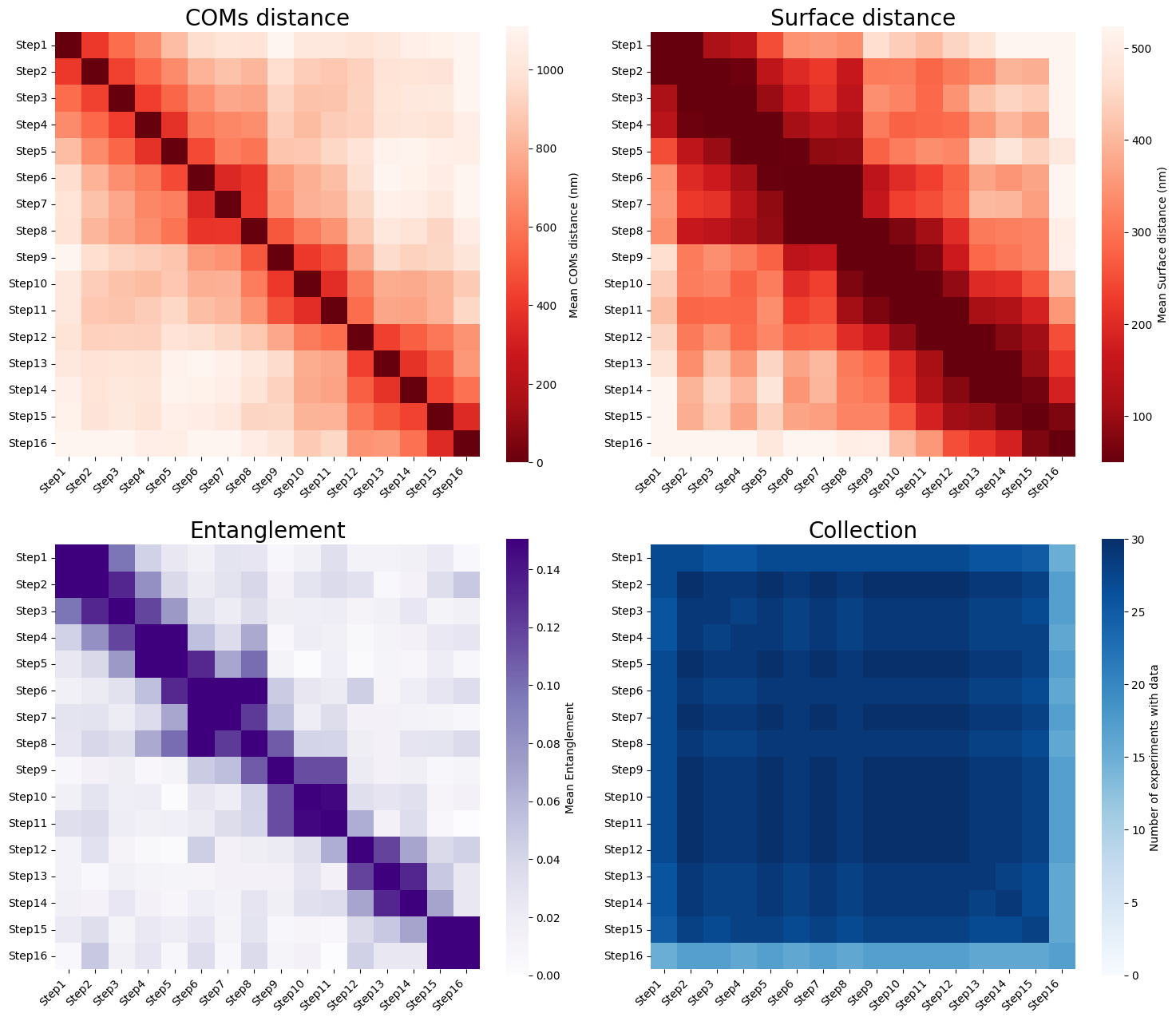
heatmap for COMs distances, surface distance, entanglement and collection

Plot mean ensemble matrices for varied spatial measuraments available in CIMA, namely:

coms_distance: The distance score (DS) between two chromosomal segments is calculated as the spatial distance between the centers of mass of each chromosomal segment of the OligoSTORM density maps.

surface_distance: The surface distance score (SDS) between two chromosomal segments is calculated as the minimal spatial distance between the chromosomal segment of the OligoSTORM density maps.

entanglement: The entanglement score (ES) between two chromosomal segments is calculated as the fraction of overlapping voxels within the optimal iso-contour threshold with respect to the smaller of the two density maps.

collection: the N for any given pairs of imaged segments.

fig, ax = plt.subplots(nrows = 2, ncols = 2, figsize = (15,13))

sns.heatmap(
    data = mean_combined_mats["coms_distance"], 
    ax = ax[0,0],
    cmap = "Reds_r",
    square = True,
    vmax = np.nanquantile(mean_combined_mats["coms_distance"], 0.95),
    cbar_kws = {"shrink" : 0.95, "label" : "Mean COMs distance (nm)"},
    xticklabels = list(tp_names.values()),
    yticklabels = list(tp_names.values()),
    )
ax[0,0].set_xticklabels(ax[0,0].get_xticklabels(), rotation = 45, ha= "right")
ax[0,0].set_title("COMs distance", fontsize = 20)

sns.heatmap(
    data = mean_combined_mats['surface_distance'],
    ax=ax[0,1],
    cmap='Reds_r',
    square=True,
    vmin=50.,
    vmax=np.nanquantile(mean_combined_mats["surface_distance"], 0.95),
    cbar_kws = {"shrink" : 0.95, "label" : "Mean Surface distance (nm)"},
    xticklabels = list(tp_names.values()),
    yticklabels = list(tp_names.values()),
    )
ax[0,1].set_xticklabels(ax[0,1].get_xticklabels(), rotation = 45, ha= "right")
ax[0,1].set_title("Surface distance", fontsize = 20)

sns.heatmap(
    data = mean_combined_mats['entanglement'],
    ax = ax[1,0],
    cmap = "Purples",
    square = True,
    vmin = 0.0,
    vmax=np.nanquantile(mean_combined_mats["entanglement"], 0.9),
    cbar_kws = {"shrink" : 0.95, "label" : "Mean Entanglement"},
    xticklabels = list(tp_names.values()),
    yticklabels = list(tp_names.values()),
    )
ax[1,0].set_xticklabels(ax[1,0].get_xticklabels(), rotation = 45, ha= "right")
ax[1,0].set_title("Entanglement", fontsize = 20)

sns.heatmap(
    data = collection_combined_mats['coms_distance'],
    ax=ax[1,1],
    cmap='Blues',
    square=True,
    vmin=0.0,
    vmax=np.nanmax(collection_combined_mats["coms_distance"]),
    cbar_kws = {"shrink" : 0.95, "label" : "Number of experiments with data"},
    xticklabels = list(tp_names.values()),
    yticklabels = list(tp_names.values()),
    )
ax[1,1].set_xticklabels(ax[1,1].get_xticklabels(), rotation = 45, ha= "right")
ax[1,1].set_title('Collection', fontsize = 20)

plt.tight_layout()

if save_plots:
    filename = f'summary_heatmaps_coms_surface_entanglement' + (f"_{file_suffix}" if file_suffix != '' else '') + '.pdf'
    plot_filename = Path(plots_folder, filename)
    print(f"Saving plots to: {plot_filename}")
    plt.savefig(plot_filename, **plot_opts)
    del filename, plot_filename
else:
    plt.show()

plt.close()

del fig, ax

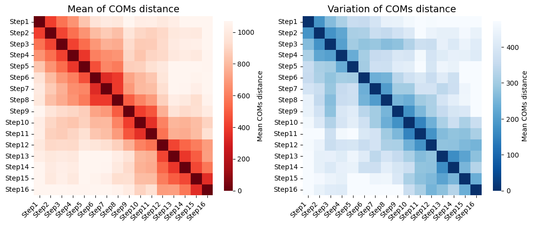
heatmap for mean and variation of COMs distance

mean_vs_variance_heatmap(mean_matrix = mean_combined_mats["coms_distance"],
                         std_matrix = std_combined_mats["coms_distance"],
                         nice_name = "COMs distance",
                         timepoint_name_dict = tp_names)

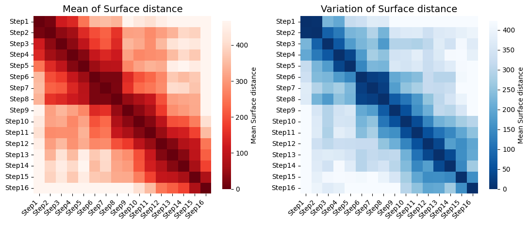
heatmap for mean and variation of surface distance

mean_vs_variance_heatmap(mean_matrix = mean_combined_mats["surface_distance"],
                         std_matrix = std_combined_mats["surface_distance"],
                         nice_name = "Surface distance",
                         timepoint_name_dict = tp_names)

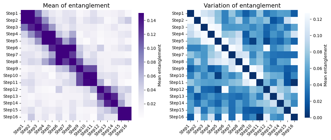
heatmap for mean and variation of entnglement

mean_vs_variance_heatmap(mean_matrix = mean_combined_mats["entanglement"],
                         std_matrix = std_combined_mats["entanglement"],
                         nice_name = "entanglement", 
                         timepoint_name_dict = tp_names,
                         hm_color = "Purples")

Plot the variation matrices for each spatial feature analysed

Back to the section index

fig, ax = plt.subplots(nrows = 2, ncols = 2, figsize = (15,13))

sns.heatmap(
    data = std_combined_mats["coms_distance"], 
    ax = ax[0,0],
    cmap = "Blues_r",
    square = True,
    vmax = np.nanquantile(std_combined_mats["coms_distance"], 0.95),
    cbar_kws = {"shrink" : 0.95, "label" : "Mean COMs distance (nm)"},
    xticklabels = list(tp_names.values()),
    yticklabels = list(tp_names.values()),
    )
ax[0,0].set_xticklabels(ax[0,0].get_xticklabels(), rotation = 45, ha= "right")
ax[0,0].set_title("COMs distance", fontsize = 20)

sns.heatmap(
    data = std_combined_mats["surface_distance"], 
    ax = ax[0,1],
    cmap = "Blues_r",
    square = True,
    vmax = np.nanquantile(std_combined_mats["surface_distance"], 0.95),
    cbar_kws = {"shrink" : 0.95, "label" : "Mean Surface distance (nm)"},
    xticklabels = list(tp_names.values()),
    yticklabels = list(tp_names.values()),
    )
ax[0,1].set_xticklabels(ax[0,1].get_xticklabels(), rotation = 45, ha= "right")
ax[0,1].set_title("Surface distance", fontsize = 20)

sns.heatmap(
    data = std_combined_mats["entanglement"], 
    ax = ax[1,0],
    cmap = "Blues_r",
    square = True,
    vmax = np.nanquantile(std_combined_mats["entanglement"], 0.95),
    cbar_kws = {"shrink" : 0.95, "label" : "Mean Entanglement"},
    xticklabels = list(tp_names.values()),
    yticklabels = list(tp_names.values()),
    )
ax[1,0].set_xticklabels(ax[1,0].get_xticklabels(), rotation = 45, ha= "right")
ax[1,0].set_title("Entanglement", fontsize = 20)

ax[-1, -1].axis('off')

if save_plots:
    filename = f'variation_heatmap_allfeatures' + (f"_{file_suffix}" if file_suffix != '' else '') + '.pdf'
    plot_filename = Path(plots_folder, filename)
    print(f"Saving plots to: {plot_filename}")
    plt.savefig(plot_filename, **plot_opts)
    del filename, plot_filename
else:
    plt.show()

plt.close()

del fig, ax