5 - Comparison with orthogonal methods
Description: This notebook contains an example on how to read SRX localization data (in csv format) and extract spatial features to compare with other orthogonal methods, in this case HiC.
The following index has links to the different sections of the notebook. Some sections may have additional indexes to access the subparts.
If you are using VS Code to visualize the notebook, the links will not work. This is due to how VC Code render the notebook. To navigate the notebook use the outline panel. To know more about it, check this link.
Content:
Next notebook to run:
Morphological feature extraction
Library imports and functions
import re
from pathlib import Path
from collections import defaultdict

import numpy as np
import matplotlib.pyplot as plt
from matplotlib.colors import LinearSegmentedColormap
from matplotlib import colormaps
import seaborn as sns
import pandas as pd
from scipy.stats import pearsonr

from cima.parsers.parser_csv import CSVParser
from cima.utils.walk_features import convertToMatrix, convertToFreq, getSegmentFeatures
from cima.utils.matrices_comparison import pearson_corr, scc, spearman_corr
from cima.segments.segment_gaussian import TransformBlurrer

# Set the maximum number of rows to display in the output
pd.options.display.max_rows = 999

# Set the options for saving the plots
plot_opts = {"dpi": 300, "bbox_inches": 'tight', "transparent": True}

# Labels for the plots of the features, so they look nice
plot_labels={
    "volume":"Volume ($nm^3$)",
    "area":"Area ($nm^2$)",
    "sphericity":"Sphericity",
    "sphericity_bribiesca":"Sphericity Bribiesca",
    "density_kb":"Density (blink/bp)",
    "density":"Density (blink/$nm^3$)",
    "compaction":"Genomic compactness (bp/$nm^3$)",
    "solidity":"Solidity",
    "radius_of_gyration":"Radius of gyration",
    "point_cloud_ellipticity":"Ellipticity"
    }

# When showing dataframes we want that this are the first columns, so the user can manually search for them (not recomended)
first_cols = ["experimentID", "nucleusID", "chromosome", "homolog", "timepoint", "name", "flag"]

## Regular expressions to get the metadata from the filename
regex_patterns = {
    "nucleusID": re.compile(r"(?i)nuc(\d+)"), # This searches for "Nuc" or "nuc" followed by digits
    "cellID": re.compile(r"(?i)cell(\d+)"), # This searches for "Cell" or "cell" followed by digits
    "locationID" : re.compile(r"(?i)loc-?(\d+)"), # This searches for "Loc" or "loc" followed by optional hyphen and digits
    "date" : re.compile(r"(\d{4}[-\.]\d{2}[-\.]\d{2})"), # This searches for dates in the format YYYY-MM-DD or YYYY.MM.DD
    "homolog" : re.compile(r"_([ABPM01pm])"), ## Added just in case the homolog is in the filename.
    "chromosome" : re.compile(r"(?i)(chr[\d+MXY])") ## Added just in case the chromosome is in the filename.
    }

# Dictionary to change all the data types of the columns of the different dataframes, so the notebook is mor memory
# efficient.
dtype_dict = {
    "experimentID" : "string", "nucleusID" : "string", "chromosome" : "string",
    "homolog" : "string", "timepoint" : np.int16, "Name" :  "string", "flag" : "string", "segment1" : np.int16,
    "segment1_timepoint" : np.int16, "segment2_name" : "string", "flag_seg1" : "string", "segment2" : np.int16,
    "segment2_timepoint" : np.int16, "segment2_name" : "string", "flag_seg2" : "string", "coms_distance" : np.float32,
    "surface_distance" : np.float32, "entanglement" : np.float32, "volume" : np.float32,
    "area" : np.float32, "sphericity_bribiesca" : np.float32, "sphericity" : np.float32, "radius_of_gyration" : np.float32,
    "point_cloud_ellipticity" : np.float32, "point_cloud_eccentricity" : np.float32, "mvee_ellipticity" : np.float32,
    "mvee_eccentricity" : np.float32, "solidity" : np.float32, "holeless_solidity" : np.float32,
    "numerosity" : np.uint32, "compaction" : np.float32, "density" : np.float32, "density_kb" : np.float32
}

# We create a color map that goes from white to red for the HiC plots (put it in CIMA)
if "bright_red" not in colormaps:
    colormaps.register(name="bright_red", cmap=LinearSegmentedColormap.from_list("bright_red", [(1,1,1),(1,0,0)]))
# Function to get a dictionary to change dtypes from pandas (and save a bit of memory)
def get_dtype_dict(columns_list: list, dict_dtype: dict) -> dict:
    """
    Function to get a dictionary to facilitate the change of data types of pandas columns.
    This results in saving memory overall.

    Parameters
    ----------
    columns_list : list
        List of the columns in the DataFrame (you can use df_name.columns)
    dict_dtype : dict
        Dictionary with the desired data types for specific columns.

    Returns
    -------
    dict
        Dictionary with the desired data types for specific columns.
    """

    return {key: val for key,val in dict_dtype.items() if key in columns_list}
Setting some variables
In the following cell you should set up some variables for the script to run properly. Change the variables at your convenience, and then you can press “Run all” in the Jupyter Notebook.
Brief explanation of the different variables:
- work_folder: this variable is where the plots and the tsv files that the script creates will be stored.
- data_file: this variable is where the csv files to be assessed are stored.
- info_file: file that contains information about your walks, such as the chromosome, start and end of the steps. You need a columns that matches the 'timepoint' column in the csv files, to be able to show proper information.
- column_round: the column that matches the 'timepoint' column in the csv files.
- column_name: the column with the "nice" name for the steps. This will be used instead of the timepoint number. Use "" in case the information file does not have this column (in this case the name of the steps will be in the form of 'StepN' where N is an incremental number form 1 to the max number of steps).
- column_size: the column for the size of the segment. Use "" in case the information file does not have this column (in this case the notebook will calculate the size automatically of the segments according to the start and end positions in the file).
- column_start_pos: the column of the start position of the timepoint.
- column_end_pos: the column of the start position of the timepoint.
- number_of_steps_library: the number of steps in your library.
- starting_step: the step at which analysis should start.
- prec_mean_dataset: the worst precision of the three axes (usually the Z). This will be used as a blurring factor when creating the 3D maps to calculate the volumetric features.
- save_plots: save the plots into a folder or show them in the notebook.
- file_suffix: add a suffix to the different files created, in case you wish to save the results from different assessments in the same folder. It will be added as "_suffix" before the .tsv/.pdf.
The notebook will create a folder in the work_folder path called 5_comparison_with_orthogonal_methods. Inside this folder 2 subfolders will be created, one for tsvs and one for plots. Inside each folder, a sub-subfolder with the suffix name will have the plots/tsvs for that experiment.
5_comparison_with_orthogonal_methods/
|-- tsvs/
|   |-- example_tsv_SUFFIX.tsv
|-- plots/
|   |-- example_plot_SUFFIX.pdf
work_folder = "/scratch/CIMA_tutorial/"
data_folder = "/scratch/CIMA_tutorial/data/chr3"

info_file = "/scratch/CIMA_tutorial/data/chr3/Info_chr3.txt"

column_round = "Round"
column_name = "Name"
column_size = "Size(kb)"
column_chr = "Chr"
column_start_pos = "Start(hg19)"
column_end_pos = "End(hg19)"

number_of_steps_library = 16
starting_step = 6

prec_mean_dataset = 30

save_plots = False

file_suffix = "chr3"
work_folder = Path(work_folder)
data_folder = Path(data_folder)
pre_assessment_folder = Path(work_folder, "2_experimental_quality_assessment")
reconstruction_tsv_folder = Path(work_folder, "3_3D_reconstruction_assessment", "tsvs", file_suffix)

info_df = pd.read_table(Path(info_file), sep="\t")
info_df.columns = info_df.columns.str.strip() # In case there are leading or trailing spaces in the column names

info_file_dict = {
    "column_round" : column_round,
    "column_name" : column_name,
    "column_size" : column_size,
    "column_chr" : column_chr,
    "column_start_pos" : column_start_pos,
    "column_end_pos" : column_end_pos,
}

del column_round, column_name, column_size, column_chr, column_start_pos, column_end_pos, info_file
Exporting the data with CIMA
Content:
Creating the list of CIMA StructuralObject
In this cell we create a list of StructuralObjects (the main CIMA class type).
This list is the basis to do the assessment through this Jupyter Notebook.
When loading the data, we will also take out those traces or CS that did not pass the assessment in the previous notebooks.
When reading the file, it will also add some metadata gathered from the filename of the csv file:
- nucleusID: searches for "nuc" (with any combination of lower and upper case) followed by digits. If there is not a match, the default is filecount (first file read will be number 1, ...).
- cellID: searches for "cell" (with any combination of lower and upper case) followed by digits. If there is not a match, the default is filecount (first file read will be number 1, ...).
- locationID: searches for "loc" (with any combination of lower and upper case) followed by optional hyphen and digits.If there is not a match, the default is filecount (first file read will be number 1, ...).
- date: searches for dates in the format YYYY-MM-DD or YYYY.MM.DD. If there is not a match, the default is the file name.
- homolog: searches for "_" followed by A, B, M, P, m, p, 0 or 1 (only one instance of this). If there is not a match, the default is "A".
- chromosome: searches for "chr" (with any combination of lower and upper case) followed by a number, M, X or Y. If there is not a match, the default is "chrN".
# Get a list of all CSV files in the specified data folder
csv_files = list(data_folder.glob('*.csv'))

if len(csv_files) == 0:
    print("No files found, please input the correct work_folder")
else:
    print(f"Total number of files found: {len(csv_files)}")

print("Loading the experimental quality data from the CSV files")
traces_pass = pd.read_csv(Path(pre_assessment_folder, f"experimental_assessment_pass_{file_suffix}.txt"), sep="\t", names=["trace"])

print("Loading the bad flags from the CSV files")
segments_to_remove_CCC = pd.read_csv(Path(reconstruction_tsv_folder, f'segments2remove_bycccvariation_t2{("_" + file_suffix) if file_suffix != "" else ""}.tsv'), sep="\t")
if "flag" not in segments_to_remove_CCC.columns and not segments_to_remove_CCC.empty:
    print("\tCreating the 'flag' column for reconstruction-based removal")
    segments_to_remove_CCC["flag"] = segments_to_remove_CCC[["experimentID", "nucleusID", "homolog", "timepoint"]].astype(str).apply("_".join, axis=1)
    bad_flags = set(segments_to_remove_CCC["flag"].astype(str).values)
elif not segments_to_remove_CCC.empty:
    bad_flags = set(segments_to_remove_CCC["flag"].astype(str).values)
else:
    bad_flags = set()

# Get a list of metadata keys to extract from filenames
metadata_keys = ["nucleusID", "cellID", "locationID", "date", "homolog", "chromosome"]

# Initialize an empty list to store the StructuralObject instances
obj_list = []

list_of_rog = []

if len(csv_files) > 0:
    # Iterate over each file in the list of file names
    for count, filein in enumerate(csv_files, start=1):

        stem = Path(filein).stem

        if not stem in traces_pass["trace"].values:
            print(f"\tSkipping file {count}: {stem} because it did not pass the experimental quality assessment.")
            continue

        print(f"Processing file {count}: {stem}", end="\r")

        # We mine the metadata from the filename using regex patterns. If not possible, assign default values.
        # In the case of nucleus, cell and location, the default is the filecount (first file read will be number 1, ...)
        # In the case of date, if no date can be found, the filename gets used.
        # If no valid homolog denomination is found, the default value is A.
        # If no valid chromosome denomination is found, the default value is chrN.
        metadata_CIMA = {
            key: (match.group(1) if (match := regex_patterns[key].search(stem)) else default)
            for key, default in zip(metadata_keys, [count, count, count, stem, "A", "chrN"])
        }

        # Adjust the metadata for nucleus and cell (if nucleus is count, but cell is something, use the cell match in nucleus)
        if "cellID" in metadata_CIMA and metadata_CIMA["nucleusID"] == count:
            metadata_CIMA["nucleusID"] = metadata_CIMA["cellID"]

        # Set experimentID as date for consistency
        metadata_CIMA["experimentID"] = metadata_CIMA["date"]

        # Read the CSV file and create a StructuralObject instance
        objin = CSVParser.read_CSV_file(filein.as_posix(), metadata = metadata_CIMA, content_type = "srx")

        # Filter the atomList to include only the specified timepoints in the info file
        objin.atomList = objin.atomList[(objin.atomList['timepoint'] >= starting_step - 1) &
                                        (objin.atomList['timepoint'] < (starting_step + number_of_steps_library - 1))].copy()

        experiment_id = objin.metadata["experimentID"]
        nucleus_id = int(objin.metadata["nucleusID"])
        homolog = objin.metadata["homolog"]

        full_flags = (experiment_id + "_" + str(nucleus_id) + "_" +homolog + "_" + objin.atomList["timepoint"].astype(str))
        remove_mask = full_flags.isin(bad_flags)

        if remove_mask.any():
            removed_tps = objin.atomList.loc[remove_mask, "timepoint"].unique()
            # removed_tps = ",".join([tp_names[tp] for tp in removed_tps])
            # print(f"Excluding timepoints {removed_tps} in experimentID: {experiment_id}, nucleusID: {nucleus_id}, homolog: {homolog} due to poor assessment.")
            objin.atomList = objin.atomList.loc[~remove_mask].copy()

        for tp in objin.atomList["timepoint"].unique():
            # Take out the timepoint from the atomList if it has less tha 10 points
            tp_mask = objin.atomList["timepoint"] == tp
            if tp_mask.sum() < 10:
                print(f"\tExcluding timepoint {tp} in experimentID: {experiment_id}, nucleusID: {nucleus_id}, homolog: {homolog} because it has less than 10 points.")
                objin.atomList = objin.atomList.loc[~tp_mask].copy()
                continue

            map_tp = TransformBlurrer().SR_gaussian_blur(objin.get_Time_segment(tp), prec_mean_dataset, sigma_coeff=1., mode="unit")
            rog_tp = getSegmentFeatures(objin.get_Time_segment(tp), map_tp, features=["radius_of_gyration"])["radius_of_gyration"]
            list_of_rog.append(rog_tp)

        # Append the object to the list
        obj_list.append(objin)

    # Nice print to tell the user the number of objects created.
    print(f"\nTotal number of objects created: {len(obj_list)}")

    # Clean up memory by deleting some of the variables no longer needed
    del count, filein, stem, metadata_CIMA, match, objin

del csv_files, metadata_keys
del bad_flags
del experiment_id, nucleus_id, homolog, full_flags, remove_mask, tp, removed_tps, tp_mask, map_tp, rog_tp
if 'segments_to_remove_CCC' in locals():
    del segments_to_remove_CCC
Total number of files found: 33
Loading the experimental quality data from the CSV files
Loading the bad flags from the CSV files
	Creating the 'flag' column for reconstruction-based removal
	Skipping file 2: 2018-07-10_nuc04_A_chr3 because it did not pass the experimental quality assessment.
	Skipping file 5: 2018-07-10_nuc03_A_chr3 because it did not pass the experimental quality assessment.
	Excluding timepoint 19 in experimentID: 2018-09-04, nucleusID: 7, homolog: A because it has less than 10 points.
	Skipping file 26: 2018-09-04_nuc01_A_chr3 because it did not pass the experimental quality assessment.
Processing file 33: 2018-09-04_nuc06_A_chr3
Total number of objects created: 30
Checking the information file
This cells makes an adjustment in the info_df.
It checks if the column of the info_df that we will use as the link between this data frame and our walks has the same timepoints. This happens because most programs start with timepoint 0, while most information files start at timepoint 1.
This will create a new column in the dataframe that is called ‘timepoint’. This column will be modified so it has the same range as the timepoint column from the csv files.
list_of_timepoints = sorted({int(tp) for obj in obj_list for tp in obj.atomList.timepoint.unique()})
info_of_timepoints = list(map(int, info_df[info_file_dict["column_round"]].tolist()))

print(f'List of timepoints found across all objects: {list_of_timepoints}')
print(f'List of timepoints in the information file: {info_of_timepoints}\n')

if list_of_timepoints == info_of_timepoints:
    print('The timepoints found in the objects match those in the information file.')
    info_df["timepoint"] = info_df[info_file_dict["column_round"]]
elif set(list_of_timepoints).issubset(info_of_timepoints):
    print('Note: The timepoints found in the objects are a subset of those in the information file. Not all timepoints are present.')
    info_df["timepoint"] = info_df[info_file_dict["column_round"]]
elif list_of_timepoints == [x - 1 for x in info_of_timepoints]:
    print('Note: The column for the information file that has the timepoint is offset by 1 compared to the objects, adjusting accordingly.')
    info_df["timepoint"] = info_df[info_file_dict["column_round"]] - 1
elif set(list_of_timepoints).issubset({x - 1 for x in info_of_timepoints}):
    print('Note: The timepoints found in the objects are a subset of those in the information file, which are offset by 1 compared to the objects. Adjusting accordingly.')
    info_df["timepoint"] = info_df[info_file_dict["column_round"]] - 1
else:
    print('Warning: The timepoints found in the objects do not match those in the information file.')

if info_file_dict["column_size"] == "":
    print("Calculating size column from start and end positions...")
    column_size = "size"
    info_file_dict["column_size"] = column_size
    info_df[column_size] = info_df[info_file_dict["column_end_pos"]] - info_df[info_file_dict["column_start_pos"]]

if info_file_dict["column_name"] == "":
    print("Setting name column from round numbers...")
    info_file_dict["column_name"] = "name"
    info_df["name"] = [f"Step{i}" for i in range(1, info_df.shape[0]+1)]

tp_names = info_df.set_index("timepoint")[info_file_dict["column_name"]].to_dict()

del list_of_timepoints, info_of_timepoints
List of timepoints found across all objects: [5, 6, 7, 8, 9, 10, 11, 12, 13, 14, 15, 16, 17, 18, 19, 20]
List of timepoints in the information file: [6, 7, 8, 9, 10, 11, 12, 13, 14, 15, 16, 17, 18, 19, 20, 21]

Note: The column for the information file that has the timepoint is offset by 1 compared to the objects, adjusting accordingly.
Creating a color palette and the results folders for the tsv and plot files
Here we create a color palette automatically based on the different experiment ID found across the files. Experiment IDs are usually the date of the experiment. This allows to easily check for a possible batch effect.
We also create the folders were to store the results.
# Define the color palette for experiments. Use the date or the experimentID (date) as the key.
color_palette = {exp_date: color for exp_date, color in zip(
    # We get a set of unique dates from the metadata of the objects
    set([file.metadata["experimentID"] for file in obj_list]),
    # We assign a color from the tab10 palette for each unique date
    sns.color_palette("tab10", n_colors=len(set([file.metadata["experimentID"] for file in obj_list])))
)}

# This palette is fixed for the current experiments used in the tutorial, which aim to reproduce the figures in the CIMA paper.
color_palette = {'2018-01-11':"#a6cee3" ,'2018-06-28':'#1f78b4', '2018-07-10':'#b2df8a', '2018-09-04':'#33a02c'}

# Create the folders to save the results. If the folders already exist, do not raise an error.
tsv_folder = Path(work_folder, "5_comparison_with_orthogonal_methods", "tsvs", file_suffix)
tsv_folder.mkdir(parents=True, exist_ok=True)

plots_folder = Path(work_folder, "5_comparison_with_orthogonal_methods", "plots", file_suffix)
plots_folder.mkdir(parents=True, exist_ok=True)
Proximity frequency ensemble matrix
Content:
Loading the distance data and calculating the mean distance matrix from all the walks
distance_folder = Path(work_folder, "4_distance_extraction", "tsvs", file_suffix)
distance_file = Path(distance_folder, f'spatial_features_{prec_mean_dataset}{("_" + file_suffix) if file_suffix != "" else ""}.tsv')

dataframe_spatialfeatures = pd.read_table(distance_file, sep="\t")

if "flag" not in dataframe_spatialfeatures.columns:
    dataframe_spatialfeatures["flag"] = dataframe_spatialfeatures[["experimentID", "nucleusID", "homolog"]].astype(str).apply("_".join, axis=1)

if "flag_seg1" not in dataframe_spatialfeatures.columns:
    dataframe_spatialfeatures["flag_seg1"] = dataframe_spatialfeatures[["experimentID", "nucleusID", "homolog", "segment1_timepoint"]].astype(str).apply("_".join, axis=1)

if "flag_seg2" not in dataframe_spatialfeatures.columns:
    dataframe_spatialfeatures["flag_seg2"] = dataframe_spatialfeatures[["experimentID", "nucleusID", "homolog", "segment2_timepoint"]].astype(str).apply("_".join, axis=1)

dataframe_spatialfeatures = dataframe_spatialfeatures.astype(get_dtype_dict(dataframe_spatialfeatures.columns.to_list(), dtype_dict))
mean_combined_mats = {}
std_combined_mats = {}
collection_combined_mats = {}

for feat in ['coms_distance', 'surface_distance', 'entanglement']:

    print(f"Working on feature: {feat}...")

    combined_ent_mat0=[]

    for f in dataframe_spatialfeatures.flag.unique().tolist():

        # print(f"\tProcessing flag: {f}...")

        mat = convertToMatrix(pairs_features_df = dataframe_spatialfeatures[dataframe_spatialfeatures.flag == f],
                              value = feat,
                              cluss = np.array(info_df.timepoint.tolist()))

        mat = mat.astype(np.float64)
        combined_ent_mat0.append(mat)

    mean_combined_mats[feat] = np.nanmean(combined_ent_mat0, axis=0)
    std_combined_mats[feat] = np.nanstd(combined_ent_mat0, axis=0)
    collection_combined_mats[feat] = (np.invert(np.isnan(combined_ent_mat0))).sum(axis=0)

    # Take out rows/columns that contain 1 or more NaN values
    mean_combined_mats[feat] = mean_combined_mats[feat][~np.isnan(mean_combined_mats[feat]).any(axis=1)][:, ~np.isnan(mean_combined_mats[feat]).any(axis=0)]

    std_combined_mats[feat] = std_combined_mats[feat][~np.isnan(std_combined_mats[feat]).any(axis=1)][:, ~np.isnan(std_combined_mats[feat]).any(axis=0)]

    print(f"Working on feature: {feat}... Done!")

del feat, combined_ent_mat0, f, mat
Working on feature: coms_distance...
Working on feature: coms_distance... Done!
Working on feature: surface_distance...
Working on feature: surface_distance... Done!
Working on feature: entanglement...
Working on feature: entanglement... Done!
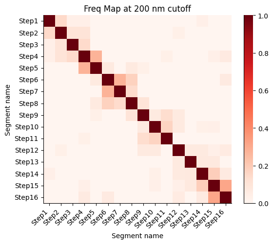
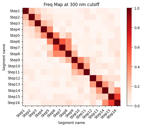
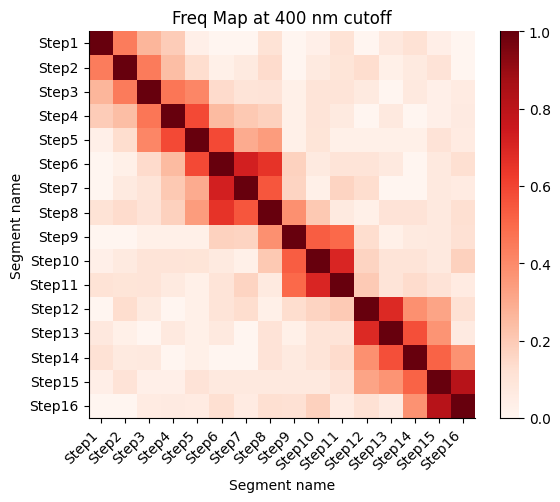
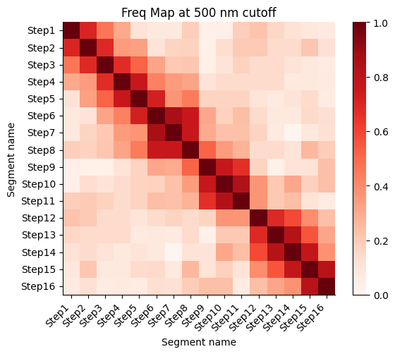
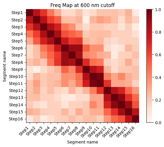
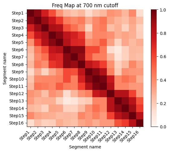
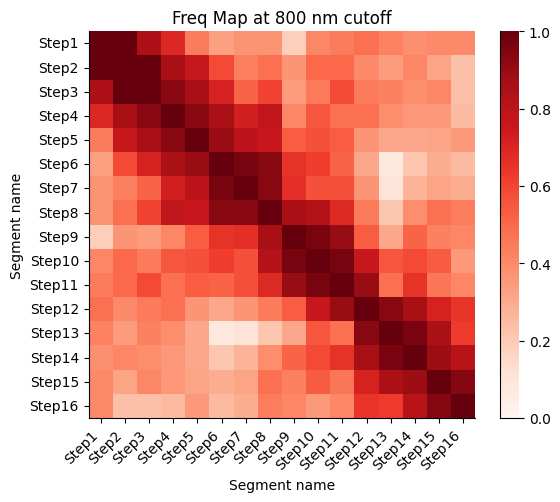
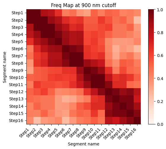
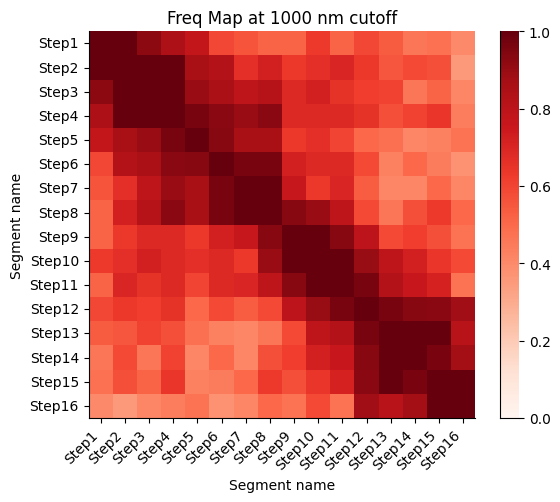
Frequency map generated from the different walks
Calculate the proximity frequency matrix for the walk-ensemble at diffrent distance cutoffs. This cutoffs should be chosen based on the radius of gyration across the different samples.
The proximity frequencies is calculated as the number of pairwise segments in which the distance between them is lower than a given cutoff normalized by the number of collected segments.
q1, q3 = np.quantile(list_of_rog, [0.25, 0.75])
iqr = q3 - q1
min_rog = q1 - 1.5 * iqr
max_rog = q3 + 1.5 * iqr

low_limit = 2 * np.nanmax([int(min_rog/100)*100, 100])
high_limit = 2 * (int(max_rog/100)*100) + 1

freqmap_dict={}

for cutoff in range(low_limit, high_limit, 100):

    print(f"Working on cut-off: {cutoff}")

    freq_temp = [convertToFreq(pairs_features_df = dataframe_spatialfeatures,
                               value = "coms_distance",
                               filename = f,
                               cluss = np.arange(starting_step - 1,starting_step + number_of_steps_library - 1),
                               cut0ff = cutoff) for f in dataframe_spatialfeatures["flag"].unique()]

    freqmap = np.stack(freq_temp, axis=0)
    freqmap = np.nansum(freqmap, axis=0)
    freqmap = np.divide(freqmap, collection_combined_mats["coms_distance"])

    fig, ax = plt.subplots(1, 1, figsize=(6, 5))  # 1 row, 1 columns

    # First heatmap, non-normalized
    sns.heatmap(
        data = freqmap,
        ax = ax,
        cmap='Reds',
        square=True,
        vmin=0,
        vmax=1,
        xticklabels=list(tp_names.values()),
        yticklabels=list(tp_names.values()),
        )
    ax.set_xlabel("Segment name")
    ax.set_xticklabels(ax.get_xticklabels(), rotation=45, ha='right')
    ax.set_ylabel("Segment name")
    ax.set_title(f'Freq Map at {cutoff} nm cutoff')

    sns.despine()
    plt.tight_layout()

    if save_plots:
        filename = f'contact_map_coms_distance_{cutoff}nm_cutoff' + (f"_{file_suffix}" if file_suffix != '' else '') + '.pdf'
        plot_filename = Path(plots_folder, filename)
        print(f"Saving plots to: {plot_filename}")
        plt.savefig(plot_filename, **plot_opts)
        del filename, plot_filename
    else:
        plt.show()
    plt.close()

    freqmap_dict[cutoff] = freqmap

del cutoff, freq_temp, freqmap, fig, ax
Working on cut-off: 200
Working on cut-off: 300
Working on cut-off: 400
Working on cut-off: 500
Working on cut-off: 600
Working on cut-off: 700
Working on cut-off: 800
Working on cut-off: 900
Working on cut-off: 1000
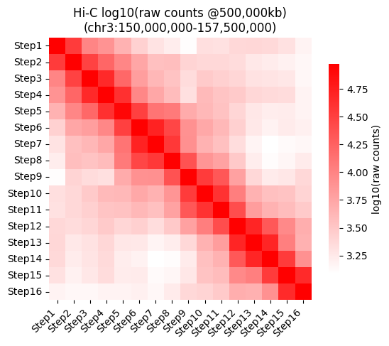
Loading the HiC data we will use for comparison
To be able to load properly the HiC matrix we need to know the resolution, the chromosome and where to start and end the matrix.
We can extract all this data from the info file.
The resolution is the step size
The chromosome is the chromosome we are imaging
The start is the smallest coordinate of the starting coordinates (the start coordinate of the first step)
The end is the biggest coordinate of the ending coordinates (the ending coordinate of the last step)
resolution2use = info_df[info_file_dict["column_size"]].unique()[0]

chrom2use = info_df[info_file_dict['column_chr']].unique()[0]

start_walk = info_df[info_file_dict["column_start_pos"]].min()
end_walk = info_df[info_file_dict["column_end_pos"]].max()
The example shown here is when using hicstraw to extract data from .hic files. If you want to use a cooler, please follow the example of the next cell (uncomment everything on that cell and comment the content of this cell)
# This HiC corresponds to the one in PLOSGEN NIR,FARABELLA,2018

# Important!!!!! CIMA does not have hicstraw by default.
try:
    import hicstraw
except ImportError:
    print("\033[91mWARNING!\033[0m")
    print("hicstraw is not installed. Hi-C related functions will not work. Please install hicstraw if you need Hi-C functionality.")

hic = hicstraw.HiCFile("/scratch/CIMA_tutorial/data/ENCFF768UBD.hic")

chrs_length_hic_dict = {c.name : c.length for c in hic.getChromosomes()}

if chrom2use not in chrs_length_hic_dict:
    try:
        chrom2use = chrom2use.replace("chr", "")
        if chrom2use not in chrs_length_hic_dict:
            raise ValueError(f"Chromosome {chrom2use} not found in Hi-C file. Available chromosomes: {list(chrs_length_hic_dict.keys())}")
    except Exception as e:
        print(f"\033[91mERROR:\033[0m Chromosome {chrom2use} not found in Hi-C file. Available chromosomes: {list(chrs_length_hic_dict.keys())}")
        raise e

resolutions = hic.getResolutions()

if resolution2use not in resolutions:
    try:
        resolution2use = resolution2use * 1000
        if resolution2use not in resolutions:
            raise ValueError(f"Resolution {resolution2use} not found in Hi-C file. Available resolutions: {resolutions}")
    except Exception as e:
        print(f"\033[91mERROR:\033[0m Resolution {resolution2use} not found in Hi-C file. Available resolutions: {resolutions}")
        raise e

start_walk = int(np.trunc(start_walk / (resolution2use))) * resolution2use
start_walk = np.max([start_walk, 0])

end_walk = int(np.ceil((end_walk - resolution2use/2) / resolution2use)) * resolution2use - resolution2use
end_walk = np.min([end_walk, [chrom.length for chrom in hic.getChromosomes() if chrom.name == chrom2use][0]])

selected_hic_map = {}

selected_hic_map["raw_counts"] = hic.getMatrixZoomData(chrom2use, chrom2use, "observed", "NONE", "BP", resolution2use).getRecordsAsMatrix(start_walk, end_walk, start_walk, end_walk)
selected_hic_map["log10_raw_counts"] = np.log10(selected_hic_map["raw_counts"]+1)

selected_hic_map["normalized_counts"] = hic.getMatrixZoomData(chrom2use, chrom2use, "observed", "VC", "BP", resolution2use).getRecordsAsMatrix(start_walk, end_walk, start_walk, end_walk)
selected_hic_map["log10_normalized_counts"] = np.log10(selected_hic_map["normalized_counts"]+1)

del hic, chrs_length_hic_dict, resolutions
Example when using cooler.
This code is not fully tested. There may be errors regarding the chromosome format or the resolution.
# # Important!!!!! CIMA does not have cooler by default.
# try:
#     import cooler
# except ImportError:
#     print("\033[91mWARNING!\033[0m")
#     print("cooler is not installed. Hi-C related functions will not work. Please install cooler if you need Hi-C functionality.")

# cool_file = cooler.Cooler("/home/imaceda-iit.local.old/intactHiC/ENCFF768UBD_10kb.cool")

# start_walk = int(np.trunc(start_walk / (resolution2use * 1000))) * resolution2use*1000
# start_walk = np.max([start_walk, 0])

# end_walk = int(np.ceil((end_walk - resolution2use*1000/2) / (resolution2use * 1000))) * resolution2use*1000
# end_walk = np.min([end_walk, cool_file.chromsizes[chrom2use]])

# selected_hic_map = {}

# selected_hic_map["raw_counts"] = cool_file.matrix(balance=False).fetch(f"16:{start_walk}-{end_walk}")
# selected_hic_map["log10_raw_counts"] = np.log10(selected_hic_map["raw_counts"]+1)

# selected_hic_map["normalized_counts"] = cool_file.matrix(balance=True).fetch(f"16:{start_walk}-{end_walk}")
# selected_hic_map["log10_normalized_counts"] = np.log10(selected_hic_map["normalized_counts"]+1)

# del cool_file
Heatmap for the raw counts at the given resolution.
g = sns.heatmap(data = selected_hic_map["log10_raw_counts"], cmap="bright_red", square=True,
                vmax=np.nanquantile(selected_hic_map["log10_raw_counts"], 0.95),
                cbar_kws={"shrink": 0.8, "label": "log10(raw counts)"},
                xticklabels=list(tp_names.values()),
                yticklabels=list(tp_names.values()))

plt.setp(g.get_xticklabels(), rotation=45, ha='right')
plt.title(f"Hi-C log10(raw counts @{resolution2use:,}kb)\n(chr{chrom2use}:{start_walk:,}-{end_walk:,})")

if save_plots:
    filename = f'hi_c_raw_counts_{start_walk}_{end_walk}' + (f"_{file_suffix}" if file_suffix != '' else '') + '.pdf'
    plot_filename = Path(plots_folder, filename)
    print(f"Saving plots to: {plot_filename}")
    plt.savefig(plot_filename, **plot_opts)
    del filename, plot_filename
else:
    plt.show()

plt.close()

del g
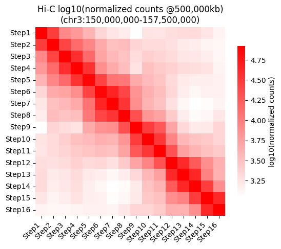
Heatmap for the normalized counts at the given resolution.
g = sns.heatmap(data = selected_hic_map["log10_normalized_counts"], cmap="bright_red", square=True,
                vmax=np.nanquantile(selected_hic_map["log10_normalized_counts"], 0.95),
                cbar_kws={"shrink": 0.8, "label": "log10(normalized counts)"},
                xticklabels=list(tp_names.values()),
                yticklabels=list(tp_names.values()))

plt.setp(g.get_xticklabels(), rotation=45, ha='right')
plt.title(f"Hi-C log10(normalized counts @{resolution2use:,}kb)\n(chr{chrom2use}:{start_walk:,}-{end_walk:,})")

if save_plots:
    filename = f'hi_c_normalized_counts_{start_walk}_{end_walk}' + (f"_{file_suffix}" if file_suffix != '' else '') + '.pdf'
    plot_filename = Path(plots_folder, filename)
    print(f"Saving plots to: {plot_filename}")
    plt.savefig(plot_filename, **plot_opts)
    del filename, plot_filename
else:
    plt.show()

plt.close()

del g
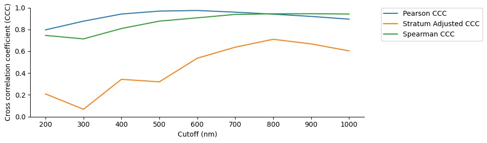
Compare the HiC and proximity frequency ensembl matrices
To do the comparison we use pearson correlation, stratum adjusted correlation and spearman correlation to compare the log10(normalized counts) of the HiC matrix with the frequency map ensembl matrix.
As we calculate the frequency map over different cut-offs we do this correlations along this different cut-offs and plot them.
ccc_df = defaultdict(list)

for cutoff,fr_map in freqmap_dict.items():

    if "zscore" in str(cutoff):
        continue

    corr_pers = pearson_corr(selected_hic_map["log10_normalized_counts"], fr_map)
    corr_scc = scc(selected_hic_map["log10_normalized_counts"], fr_map)
    corr_sp = spearman_corr(selected_hic_map["log10_normalized_counts"], fr_map)

    ccc_df["cutoff"].append(cutoff)
    ccc_df["ccc_pearson"].append(corr_pers)
    ccc_df["ccc_stratum_adjusted"].append(corr_scc)
    ccc_df["ccc_spearman"].append(corr_sp)

ccc_df = pd.DataFrame(ccc_df)
display(ccc_df)

plt.figure(figsize=(10, 3))

sns.lineplot(data = ccc_df, x="cutoff", y="ccc_pearson", label='Pearson CCC')
sns.lineplot(data = ccc_df, x="cutoff", y="ccc_stratum_adjusted", label='Stratum Adjusted CCC')
sns.lineplot(data = ccc_df, x="cutoff", y="ccc_spearman", label='Spearman CCC')

plt.ylim(0, 1)
plt.xlabel('Cutoff (nm)')
plt.ylabel('Cross correlation coefficient (CCC)')
plt.xticks(ticks=ccc_df["cutoff"], labels=ccc_df["cutoff"])
plt.legend(bbox_to_anchor=(1.05, 1), loc=2, borderaxespad=0.)

sns.despine()
plt.tight_layout()

if save_plots:
    filename = f'lineplot_correlations_hic_proximity_freq' + (f"_{file_suffix}" if file_suffix != '' else '') + '.pdf'
    plot_filename = Path(plots_folder, filename)
    print(f"Saving plots to: {plot_filename}")
    plt.savefig(plot_filename, **plot_opts)
    del filename, plot_filename
else:
    plt.show()

plt.close()

del cutoff, fr_map, corr_pers, corr_scc, corr_sp
| cutoff | ccc_pearson | ccc_stratum_adjusted | ccc_spearman | |
|---|---|---|---|---|
| 0 | 200 | 0.796399 | 0.209564 | 0.745509 |
| 1 | 300 | 0.876046 | 0.068205 | 0.713338 |
| 2 | 400 | 0.941393 | 0.342750 | 0.808521 |
| 3 | 500 | 0.968344 | 0.319825 | 0.876429 |
| 4 | 600 | 0.974000 | 0.536663 | 0.906745 |
| 5 | 700 | 0.958406 | 0.637439 | 0.937886 |
| 6 | 800 | 0.940291 | 0.709841 | 0.943325 |
| 7 | 900 | 0.919643 | 0.667689 | 0.944305 |
| 8 | 1000 | 0.894271 | 0.603599 | 0.941211 |
lineplot of the 3 different measures for correlation between the HiC and the ensembl across the different cut-offs
fig, axes = plt.subplots(3, 1, figsize=(10, 10), sharey=True)

# Panel A - CCC Pearson
sns.lineplot(data = ccc_df, x="cutoff", y="ccc_pearson", color="tab:blue", ax=axes[0])
# Add a vertical line at the highest CCC Pearson value
max_value = ccc_df.loc[ccc_df["ccc_pearson"].idxmax(), "cutoff"]
axes[0].axvline(x=max_value, color='gray', linestyle='--', alpha = 0.25)
axes[0].set_title("Pearson CCC")
axes[0].set_xlabel("Cutoff (nm)")
axes[0].set_xticks(ccc_df["cutoff"])
axes[0].set_ylabel("Cross correlation coefficient (CCC)")
axes[0].set_ylim(0, 1)
sns.despine(ax=axes[0])

# Panel B - SCC
sns.lineplot(data = ccc_df, x="cutoff", y="ccc_stratum_adjusted", color="tab:orange", ax=axes[1])
max_value = ccc_df.loc[ccc_df["ccc_stratum_adjusted"].idxmax(), "cutoff"]
axes[1].axvline(x=max_value, color='gray', linestyle='--', alpha = 0.25)
axes[1].set_title("Stratum-adjusted CCC")
axes[1].set_xlabel("Cutoff (nm)")
axes[1].set_xticks(ccc_df["cutoff"])
axes[1].set_ylabel("Cross correlation coefficient (CCC)")
sns.despine(ax=axes[1])

# Panel C - Spearman CCC
sns.lineplot(data = ccc_df, x="cutoff", y="ccc_spearman", color="tab:green", ax=axes[2])
max_value = ccc_df.loc[ccc_df["ccc_spearman"].idxmax(), "cutoff"]
axes[2].axvline(x=max_value, color='gray', linestyle='--', alpha = 0.25)
axes[2].set_title("Spearman CCC")
axes[2].set_xlabel("Cutoff (nm)")
axes[2].set_xticks(ccc_df["cutoff"])
axes[2].set_ylabel("Cross correlation coefficient (CCC)")
sns.despine(ax=axes[2])

plt.tight_layout()
if save_plots:
    filename = f'lineplot_correlations_hic_proximity_freq_separated' + (f"_{file_suffix}" if file_suffix != '' else '') + '.pdf'
    plot_filename = Path(plots_folder, filename)
    print(f"Saving plots to: {plot_filename}")
    plt.savefig(plot_filename, **plot_opts)
    del filename, plot_filename
else:
    plt.show()
plt.close()

del fig, axes, max_value
# del ccc_df
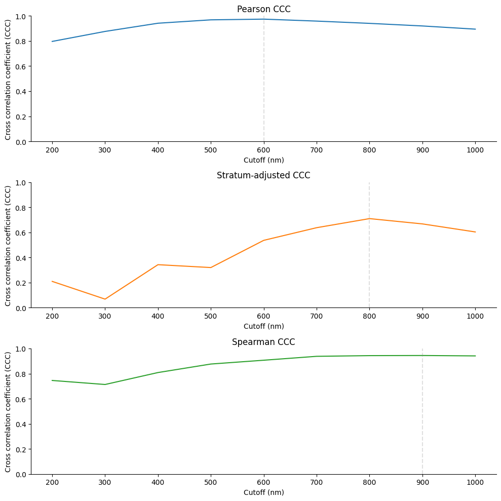
ccc_df[ccc_df["cutoff"].isin([600, 900, 1000])]
| cutoff | ccc_pearson | ccc_stratum_adjusted | ccc_spearman | |
|---|---|---|---|---|
| 4 | 600 | 0.974000 | 0.536663 | 0.906745 |
| 7 | 900 | 0.919643 | 0.667689 | 0.944305 |
| 8 | 1000 | 0.894271 | 0.603599 | 0.941211 |
Correlation between the log10(normalized counts) and the COMs mean distance matrix
corr_pers = pearson_corr(selected_hic_map["log10_normalized_counts"], mean_combined_mats['coms_distance'])
corr_scc = scc(selected_hic_map["log10_normalized_counts"], mean_combined_mats['coms_distance'])
corr_sp = spearman_corr(selected_hic_map["log10_normalized_counts"], mean_combined_mats['coms_distance'])

print(f"Pearson correlation coefficient between log10(HiC normalized counts) and COMs distance: {corr_pers:.4f}")
print(f"Spearman correlation coefficient between log10(HiC normalized counts) and COMs distance: {corr_sp:.4f}")
print(f"Stratum adjusted correlation coefficient between log10(HiC normalized counts) and COMs distance: {corr_scc:.4f}")

del corr_pers, corr_scc, corr_sp
Pearson correlation coefficient between log10(HiC normalized counts) and COMs distance: -0.9786
Spearman correlation coefficient between log10(HiC normalized counts) and COMs distance: -0.9649
Stratum adjusted correlation coefficient between log10(HiC normalized counts) and COMs distance: -0.7004
Aggregation of the data in a common dataframe, for ease of use.
In this cell we create a dataframe to aggregate all the data.
It has the following columns:
# Initialize an empty list to store pairs
pairs_df = defaultdict(list)

# Iterate over the HiC DataFrame to create pairs
for i in range(selected_hic_map["normalized_counts"].shape[0]):
    for j in range(i, selected_hic_map["normalized_counts"].shape[1]):
        if mean_combined_mats["coms_distance"][i, j] == 0:
            continue
        pairs_df["segment1_timepoint"].append(i)
        pairs_df["segment1_coordinates"].append(start_walk + i * 500000)
        pairs_df["segment2_timepoint"].append(j)
        pairs_df["segment2_coordinates"].append(start_walk + j * 500000)
        pairs_df["HiC_raw_counts"].append(selected_hic_map["raw_counts"][i, j])
        pairs_df["HiC_log10_raw_counts"].append(selected_hic_map["log10_raw_counts"][i, j])
        pairs_df["HiC_norm_counts"].append(selected_hic_map["normalized_counts"][i, j])
        pairs_df["HiC_log10_norm_counts"].append(selected_hic_map["log10_normalized_counts"][i, j])
        pairs_df["mean_coms_distance"].append(mean_combined_mats["coms_distance"][i, j])
        pairs_df["log10_mean_coms_distance"].append(np.log10(mean_combined_mats["coms_distance"][i, j]))
        pairs_df["mean_surface_distance"].append(mean_combined_mats["surface_distance"][i, j])
        pairs_df["log10_mean_surface_distance"].append(np.log10(mean_combined_mats["surface_distance"][i, j]))
        pairs_df["std_coms_distance"].append(std_combined_mats["coms_distance"][i, j])
        pairs_df["log10_std_coms_distance"].append(np.log10(std_combined_mats["coms_distance"][i, j]))
        pairs_df["std_surface_distance"].append(std_combined_mats["surface_distance"][i, j])
        pairs_df["log10_std_surface_distance"].append(np.log10(std_combined_mats["surface_distance"][i, j]))

# Create a DataFrame from the pairs list
pairs_df = pd.DataFrame(pairs_df)

# Print the resulting DataFrame
display(pairs_df.head())

del i, j
| segment1_timepoint | segment1_coordinates | segment2_timepoint | segment2_coordinates | HiC_raw_counts | HiC_log10_raw_counts | HiC_norm_counts | HiC_log10_norm_counts | mean_coms_distance | log10_mean_coms_distance | mean_surface_distance | log10_mean_surface_distance | std_coms_distance | log10_std_coms_distance | std_surface_distance | log10_std_surface_distance | |
|---|---|---|---|---|---|---|---|---|---|---|---|---|---|---|---|---|
| 0 | 0 | 150000000 | 1 | 150500000 | 34247.0 | 4.534635 | 29843.898438 | 4.474870 | 405.966592 | 2.608490 | 12.973984 | 1.113073 | 182.401960 | 2.261030 | 4.304033 | 0.633876 |
| 1 | 0 | 150000000 | 2 | 151000000 | 9780.0 | 3.990383 | 8320.222656 | 3.920187 | 566.327643 | 2.753068 | 120.525821 | 2.081080 | 266.657895 | 2.425954 | 225.993086 | 2.354095 |
| 2 | 0 | 150000000 | 3 | 151500000 | 7661.0 | 3.884342 | 6355.332520 | 3.803207 | 669.688233 | 2.825873 | 141.021260 | 2.149285 | 314.242689 | 2.497265 | 201.462147 | 2.304193 |
| 3 | 0 | 150000000 | 4 | 152000000 | 4548.0 | 3.657916 | 3984.038086 | 3.600432 | 837.295167 | 2.922879 | 248.534453 | 2.395387 | 361.246034 | 2.557803 | 319.417996 | 2.504359 |
| 4 | 0 | 150000000 | 5 | 152500000 | 2693.0 | 3.430398 | 2230.457031 | 3.348589 | 959.167460 | 2.981894 | 345.562842 | 2.538527 | 355.398837 | 2.550716 | 334.092976 | 2.523867 |
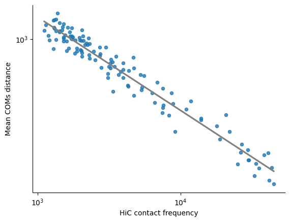
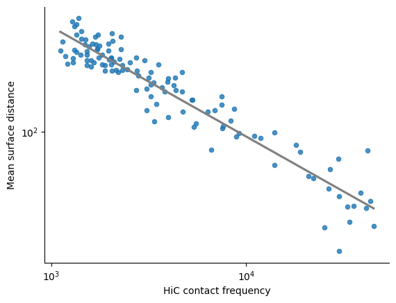
Linear regression plot between the log10(HiC normalized counts) and the log10(mean distance)
The first plot corresponds to the mean COMs distance, the second to the surface distance
print(f"Correlation between log10(HiC normalized counts) and log10(mean COMs distance): {pearsonr(pairs_df['HiC_log10_norm_counts'], pairs_df['log10_mean_coms_distance']).statistic:.4f}")
print(f"Stratum adjusted CCC between log10(HiC normalized counts) and log10(COMs distance): {scc(selected_hic_map['log10_normalized_counts'], np.log10(mean_combined_mats['coms_distance']+1e-10)):.4f}")
sns.regplot(x = pairs_df["HiC_log10_norm_counts"], y = pairs_df["log10_mean_coms_distance"], ci = 0,
            scatter_kws={'s':20}, line_kws={'color':'grey', "ls" : "-"})
xlims = plt.gca().get_xlim()
ylims = plt.gca().get_ylim()
xticks1 = np.arange(np.ceil(xlims[0]),np.floor(xlims[1])+0.1,1.0)
yticks1 = np.arange(np.ceil(ylims[0]),np.floor(ylims[1])+0.1,1.0)
plt.xticks(xticks1, [f"$10^{{ {int(xticks1[i]):0.0f} }}$" for i in range(len(xticks1))])
plt.yticks(yticks1, [f"$10^{{ {int(yticks1[i]):0.0f} }}$" for i in range(len(yticks1))])
plt.ylabel('Mean COMs distance')
plt.xlabel('HiC contact frequency')
sns.despine()
if save_plots:
    filename = f'correlation_hic_contact_frequency_mean_com_distance' + (f"_{file_suffix}" if file_suffix != '' else '') + '.pdf'
    plot_filename = Path(plots_folder, filename)
    print(f"Saving plots to: {plot_filename}")
    plt.savefig(plot_filename, **plot_opts)
    del filename, plot_filename
else:
    plt.show()
plt.close()

print()

print(f"Pearson correlation between log10(HiC normalized counts) and log10(surface distance): {pearsonr(pairs_df['HiC_log10_norm_counts'], pairs_df['log10_mean_surface_distance']).statistic:.4f}")
print(f"Stratum adjusted CCC between log10(HiC normalized counts) and log10(surface distance): {scc(selected_hic_map['log10_normalized_counts'], np.log10(mean_combined_mats['surface_distance']+1e-10)):.4f}")
sns.regplot(x = pairs_df["HiC_log10_norm_counts"], y = pairs_df["log10_mean_surface_distance"], ci = 0,
            scatter_kws={'s':20}, line_kws={'color':'grey', "ls" : "-"})
xlims = plt.gca().get_xlim()
ylims = plt.gca().get_ylim()
xticks1 = np.arange(np.ceil(xlims[0]),np.floor(xlims[1])+0.1,1.0)
yticks1 = np.arange(np.ceil(ylims[0]),np.floor(ylims[1])+0.1,1.0)
plt.xticks(xticks1, [f"$10^{int(xticks1[i]):0.0f}$" for i in range(len(xticks1))])
plt.yticks(yticks1, [f"$10^{int(yticks1[i]):0.0f}$" for i in range(len(yticks1))])
plt.ylabel('Mean surface distance')
plt.xlabel('HiC contact frequency')
sns.despine()

if save_plots:
    filename = f'correlation_hic_contact_frequency_mean_surface_distance' + (f"_{file_suffix}" if file_suffix != '' else '') + '.pdf'
    plot_filename = Path(plots_folder, filename)
    print(f"Saving plots to: {plot_filename}")
    plt.savefig(plot_filename, **plot_opts)
    del filename, plot_filename
else:
    plt.show()
plt.close()

del xlims, ylims, xticks1, yticks1
Correlation between log10(HiC normalized counts) and log10(mean COMs distance): -0.9753
Stratum adjusted CCC between log10(HiC normalized counts) and log10(COMs distance): -0.6956
Pearson correlation between log10(HiC normalized counts) and log10(surface distance): -0.9491
Stratum adjusted CCC between log10(HiC normalized counts) and log10(surface distance): -0.4620
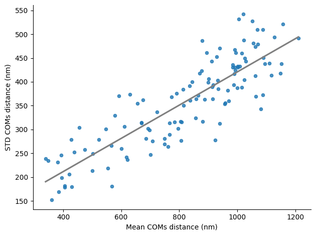
Linear regression plot between the mean COMs distance and the std COMs distance
sns.regplot(x=pairs_df["mean_coms_distance"], y=pairs_df["std_coms_distance"], ci=0,
            scatter_kws={'s':20}, line_kws={'color':'grey', "ls" : "-"})

plt.xlabel("Mean COMs distance (nm)")
plt.ylabel("STD COMs distance (nm)")

sns.despine()
plt.tight_layout()

if save_plots:
    filename = f'correlation_mean_com_distance_std_com_distance' + (f"_{file_suffix}" if file_suffix != '' else '') + '.pdf'
    plot_filename = Path(plots_folder, filename)
    print(f"Saving plots to: {plot_filename}")
    plt.savefig(plot_filename, **plot_opts)
    del filename, plot_filename
else:
    plt.show()

plt.close()