3 - 3D Reconstruction Assessment
Description: This notebook contains an example pipeline for local quality assessment of chromatin segments.
This is a pivotal steps for the reliability of downstream interpretations of volumetric chromatin tracing data. To address this, in CIMA varied methods for quality assessment that operate directly on signal of chromatin segment are available.
This assessment is the same as presented in the quality_assessment.py script from CIMA tools. If you wish to assess a huge array of files or they are located in multiple folders, please use CIMA tools over this notebook for convenience. With the script you will get the processed data needed to create most of the plots shown here.
The following index has links to the different sections of the notebook. Some sections may have additional indexes to access the subparts.
If you are using VS Code to visualize the notebook, the links may not work. This is due to how VC Code render the notebook. To navigate the notebook use the outline panel. To know more about it, check this link.
Content:
Assess by subsampling randomly over the time of aquisition to the final object (Saturation Plot)
Summary and filtering poorly assessed segments based on saturation plot
Next notebook to run is:
Distance extraction
Library imports and functions
import re
from pathlib import Path

import pandas as pd
import numpy as np
import matplotlib.pyplot as plt
import seaborn as sns

from cima.assessment.images_assessment import Cycle_assessment, Saturation_to_final_structure
from cima.parsers.parser_csv import CSVParser

# Set the maximum number of rows to display in the output
pd.options.display.max_rows = 999

# Set the options for saving the plots
plot_opts = {"dpi": 300, "bbox_inches": 'tight', "transparent": True}

# When showing dataframes we want that this are the first columns, so the user can manually search for them (not recomended)
first_cols = ["experimentID", "nucleusID", "chromosome", "homolog", "timepoint", "name", "flag"]

## Regular expressions to get the metadata from the filename
regex_patterns = {
    "nucleusID": re.compile(r"(?i)nuc(\d+)"), # This searches for "Nuc" or "nuc" followed by digits
    "cellID": re.compile(r"(?i)cell(\d+)"), # This searches for "Cell" or "cell" followed by digits
    "locationID" : re.compile(r"(?i)loc-?(\d+)"), # This searches for "Loc" or "loc" followed by optional hyphen and digits
    "date" : re.compile(r"(\d{4}[-\.]\d{2}[-\.]\d{2})"), # This searches for dates in the format YYYY-MM-DD or YYYY.MM.DD
    "homolog" : re.compile(r"_([ABPM01pm])"), ## Added just in case the homolog is in the filename.
    "chromosome" : re.compile(r"(?i)(chr[\d+MXY])") ## Added just in case the chromosome is in the filename.
    }
# Define the function to process quality assessment
def Batch_process_quality_assessment(obj_list: list,
                                     assessment_type: list = ["quality_randomsubsampling"],
                                     library_n_Hype: int = 16,
                                     start_hype: int = 5,
                                     prec_factor: int = 46,
                                     random_groups: int = 50,
                                     metaInfo: list = ["experimentID", "nucleusID", "homolog"]) -> pd.DataFrame:
    """
    Processes a list of objects to assess quality over a range of time segments using specified assessment types.

    Parameters
    ----------
    obj_list : list
        List of objects to process.
    assessment_type : list, optional
        List of assessment types to apply. Possible options are: "quality_over_time", "quality_randomsubsamplig". Default is ["quality_randomsubsampling"].
    library_n_Hype : int, optional
        Number of hyperparameters in the library. Default is 16.
    start_hype : int, optional
        Starting hyperparameter index. Default is 5.
    prec_factor : int, optional
        Precision factor. Default is 46.
    random_groups : int, optional
        Number of random groups for subsampling. Default is 50.
    metaInfo : list, optional
        List of metadata keys for the experiment ID, the nucleus ID, and the homolog. Default is ["experimentID", "nucleusID", "homolog"].

    Returns
    -------
    pd.DataFrame
        DataFrame of quality assessment scores.
    """

    dict_in = {"quality_over_time": Cycle_assessment, "quality_randomsubsampling": Saturation_to_final_structure}
    scores_list = []
    last_cols = ['assessment_type', 'cycle', 'ccc', 'nloc']

    RANGE = range(start_hype - 1, library_n_Hype - 1)

    assert all(func in dict_in for func in assessment_type), "One or more assessment types are invalid."

    for obj_counter, obj in enumerate(obj_list, start=1):
        # Extract metadata
        FOV_id = obj.metadata[metaInfo[1]]
        nucleus_ID = FOV_id
        experimentID = obj.metadata[metaInfo[0]]
        hom = obj.metadata[metaInfo[2]]
        nSteps = obj.no_of_Times()

        print(f'\033[1;4mProcessing experimentID {experimentID}, nucleusID {nucleus_ID}, hom {hom} ({obj_counter}/{len(obj_list)}).\033[0m')

        # Check if the number of steps exceeds the library hyperparameters
        if nSteps > library_n_Hype:
            print(f'\tWarning: too many segments ({nSteps}) in experimentID {experimentID}, nucleusID {nucleus_ID}, hom {hom}')
            continue

        for ts in RANGE:
            # Get the time segment
            StrObj_step = obj.get_Time_segment(timepoint=ts)
            step_name = info_df[info_df["timepoint"] == ts][info_file_dict["column_name"]].values[0]

            # Check if the segment exists
            if StrObj_step is None:
                print(f'\tWarning: missing segment {ts} in experimentID {experimentID}, nucleusID {nucleus_ID}, hom {hom}')
            else:
                # Apply the assessment function present in the assessment_type list
                for functionIN in assessment_type:
                    if functionIN == "quality_randomsubsampling":
                        scores = dict_in[functionIN](StrObj_step, prec_mean=prec_factor, selection_mode = "random", random_groups_num=random_groups, return_as_list = True)
                    else:
                        scores = dict_in[functionIN](StrObj_step, prec_mean=prec_factor)
                    # print(len(scores))
                    for line in scores:
                        # print(line)
                        scores_list.append([*line, functionIN, ts, step_name, nucleus_ID, hom, experimentID])

    dt_score = pd.DataFrame(scores_list, columns=['cycle', 'ccc', 'nloc', 'assessment_type', 'timepoint', 'name', 'nucleusID', 'homolog', 'experimentID'])

    cols = dt_score.columns.tolist()
    cols_reorder = [col for col in first_cols if col in cols] + [col for col in cols if col in last_cols]
    dt_score = dt_score[cols_reorder]

    dt_score = pd.DataFrame(dt_score)

    return dt_score
Setting some variables
In the following cell you should set up some variables for the script to run properly. Change the variables at your convenience, and then you can press “Run all” in the Jupyter Notebook.
This notebook assumes that your csv files are in SRX format.
If you want to run this notebook over multiple chromosomes/datasets, it is recomended that you do a “Clear All Outputs” and a kernel restart before running things again.
Brief explanation of the different variables:
- work_folder: this variable is where the plots and the tsv files that the script creates will be stored.
- data_file: this variable is where the csv files to be assessed are stored.
- info_file: file that contains information about your walks, such as the chromosome, start and end of the steps. You need a columns that matches the 'timepoint' column in the csv files, to be able to show proper information.
- column_round: the column that matches the 'timepoint' column in the csv files.
- column_name: the column with the "nice" name for the steps. This will be used instead of the timepoint number. Use "" in case the information file does not have this column (in this case the name of the steps will be in the form of 'StepN' where N is an incremental number form 1 to the max number of steps).
- column_size: the column for the genomic size of the segment. Use "" in case the information file does not have this column (in this case the notebook will calculate the size automatically of the segments according to the start and end positions in the file).
- column_start_pos: the column of the start position of the timepoint.
- column_end_pos: the column of the end position of the timepoint.
- number_of_steps_library: the number of steps in your library.
- starting_step: the step at which analysis should start.
- number_of_random_groups: the number of random groups when using the random subsampling method.
- save_plots: save the plots into a folder or show them in the notebook.
- file_suffix: add a suffix to the different files created, in case you wish to save the results from different assessments in the same folder. It will be added as "_suffix" before the .tsv/.pdf name. For example, 'quality_randomsubsampling.tsv' will be 'quality_randomsubsampling_SUFFIX.tsv'. It will also be used to create subfolders for data organization purposes.
The notebook will create a folder in the work_folder path called 3_3D_reconstruction_assessment. Inside this folder 2 subfolders will be created, one for plots and one for tsvs. Inside each folder, a sub-subfolder with the suffix name will have the plots/tsvs for that experiment.
3_3D_reconstruction_assessment/
|-- tsvs/
|   |-- example_tsv_SUFFIX.tsv
|-- plots/
|   |-- example_plot_SUFFIX.pdf
work_folder = "/scratch/CIMA_tutorial/"
data_folder = "/scratch/CIMA_tutorial/data/chr3"

info_file = "/scratch/CIMA_tutorial/data/chr3/Info_chr3.txt"
column_round = "Round"
column_name = "Name"
column_size = "Size(kb)"
column_start_pos = "Start(hg19)"
column_end_pos = "End(hg19)"

number_of_steps_library = 16
starting_step = 6

number_of_random_groups = 10

save_plots = False

file_suffix = "chr3"
work_folder = Path(work_folder)
data_folder = Path(data_folder)
experimental_assessment_folder = Path(work_folder, "2_experimental_quality_assessment")

info_df = pd.read_table(Path(info_file), sep="\t")
info_df.columns = info_df.columns.str.strip() # In case there are leading or trailing spaces in the column names

info_file_dict = {
    "column_round" : column_round,
    "column_name" : column_name,
    "column_size" : column_size,
    "column_start_pos" : column_start_pos,
    "column_end_pos" : column_end_pos,
}

del column_round, column_name, column_size, column_start_pos, column_end_pos, info_file
Exporting the data with CIMA
Content:
Creating the list of CIMA StructuralObjects
In this cell we create a list of StructuralObjects (the main CIMA class type).
This list is the basis to do the assessment through this Jupyter Notebook.
When reading the file, it will also add some metadata gathered from the filename of the csv file:
- nucleusID: searches for "Nuc" or "nuc" followed by digits. Only the number will be saved. If there is not a match, the default is filecount (first file read will be number 1, ...).
- cellID: searches for "Cell" or "cell" followed by digits. Only the number will be saved. If there is not a match, the default is filecount (first file read will be number 1, ...)
- locationID: searches for "Loc" or "loc" followed by optional hyphen and digits. Only the number will be saved. If there is not a match, the default is filecount (first file read will be number 1, ...)
- date: searches for dates in the format YYYY-MM-DD or YYYY.MM.DD. If there is not a match, the default is the file name.
- homolog: searches for "_" followed by A, B, M, P, m, p, 0 or 1 (only one instance of this). If there is not a match, the default is "A".
- chromosome: searches for "Chr" or "chr" followed by a number, M, X or Y. If there is not a match, the default is "chrN".
# Get a list of all CSV files in the specified data folder
csv_files = list(data_folder.glob('*.csv'))

if len(csv_files) == 0:
    print("No files found, please input the correct work_folder")
else:
    print(f"Total number of files found: {len(csv_files)}")

print("Loading the experimental quality data from the CSV files")
traces_pass = pd.read_csv(Path(experimental_assessment_folder, f"experimental_assessment_pass_{file_suffix}.txt"), sep="\t", names=["trace"])

# Get a list of metadata keys to extract from filenames
metadata_keys = ["nucleusID", "cellID", "locationID", "date", "homolog", "chromosome"]

# Initialize an empty list to store the StructuralObject instances
obj_list = []

if len(csv_files) > 0:
    # Iterate over each file in the list of file names
    for count, filein in enumerate(csv_files, start=1):

        stem = Path(filein).stem

        if not stem in traces_pass["trace"].values:
            print(f"\tSkipping file {count}: {stem} because it did not pass the experimental quality assessment.")
            continue

        print(f"Processing file {count}: {stem}")

        # We mine the metadata from the filename using regex patterns. If not possible, assign default values.
        metadata_CIMA = {
            key: (match.group(1) if (match := regex_patterns[key].search(stem)) else default)
            for key, default in zip(metadata_keys, [count, count, count, stem, "A", "chrN"])
        }

        # Adjust the metadata for nucleus and cell (if nucleus is count, but cell is something, use the cell match in nucleus)
        if "cell" in metadata_CIMA and metadata_CIMA["nucleusID"] == count:
            metadata_CIMA["nucleusID"] = metadata_CIMA["cell"]

        metadata_CIMA["nucleusID"] = int(metadata_CIMA["nucleusID"])
        metadata_CIMA["cellID"] = int(metadata_CIMA["cellID"])
        metadata_CIMA["locationID"] = int(metadata_CIMA["locationID"])

        # Set experimentID as date for consistency
        metadata_CIMA["experimentID"] = metadata_CIMA["date"]

        # Read the CSV file and create a StructuralObject instance
        objin = CSVParser.read_CSV_file(filein.as_posix(), metadata = metadata_CIMA, content_type = "srx")

        # Filter the atomList to include only the specified timepoints in the info file
        objin.atomList = objin.atomList[(objin.atomList['timepoint'] >= starting_step - 1) &
                                        (objin.atomList['timepoint'] < (starting_step + number_of_steps_library - 1))].copy()

        for tp in objin.atomList["timepoint"].unique():
            # Take out the timepoint from the atomList if it has less tha 10 points
            tp_mask = objin.atomList["timepoint"] == tp
            if tp_mask.sum() < 10:
                print(f"\tExcluding timepoint {tp} in experimentID: {metadata_CIMA['experimentID']}, nucleusID: {metadata_CIMA['nucleusID']}, homolog: {metadata_CIMA['homolog']} because it has less than 10 points.")
                objin.atomList = objin.atomList.loc[~tp_mask].copy()

        # Append the object to the list
        obj_list.append(objin)

    # Nice print to tell the user the number of objects created.
    print(f"\nTotal number of objects created: {len(obj_list)}")

    # Clean up memory by deleting some of the variables no longer needed
    del count, filein, stem, metadata_CIMA, match, objin, tp, tp_mask

del csv_files, metadata_keys, traces_pass
Total number of files found: 33
Loading the experimental quality data from the CSV files
Processing file 1: 2018-09-04_nuc03_A_chr3
	Skipping file 2: 2018-07-10_nuc04_A_chr3 because it did not pass the experimental quality assessment.
Processing file 3: 2018-07-10_nuc02_A_chr3
Processing file 4: 2018-07-10_nuc05_A_chr3
	Skipping file 5: 2018-07-10_nuc03_A_chr3 because it did not pass the experimental quality assessment.
Processing file 6: 2018-06-28_nuc07_A_chr3
Processing file 7: 2018-06-28_nuc09_A_chr3
Processing file 8: 2018-07-10_nuc11_A_chr3
Processing file 9: 2018-09-04_nuc01_B_chr3
Processing file 10: 2018-07-10_nuc06_B_chr3
Processing file 11: 2018-06-28_nuc05_B_chr3
Processing file 12: 2018-07-10_nuc06_A_chr3
Processing file 13: 2018-06-28_nuc08_A_chr3
Processing file 14: 2018-06-28_nuc05_A_chr3
Processing file 15: 2018-07-10_nuc07_A_chr3
Processing file 16: 2018-07-10_nuc01_A_chr3
Processing file 17: 2018-07-10_nuc02_B_chr3
Processing file 18: 2018-06-28_nuc01_A_chr3
Processing file 19: 2018-09-04_nuc04_A_chr3
Processing file 20: 2018-07-10_nuc04_B_chr3
Processing file 21: 2018-09-04_nuc03_B_chr3
Processing file 22: 2018-07-10_nuc03_B_chr3
Processing file 23: 2018-07-10_nuc01_B_chr3
Processing file 24: 2018-09-04_nuc07_A_chr3
	Excluding timepoint 19 in experimentID: 2018-09-04, nucleusID: 7, homolog: A because it has less than 10 points.
Processing file 25: 2018-06-28_nuc02_A_chr3
	Skipping file 26: 2018-09-04_nuc01_A_chr3 because it did not pass the experimental quality assessment.
Processing file 27: 2018-07-10_nuc10_A_chr3
Processing file 28: 2018-07-10_nuc08_A_chr3
Processing file 29: 2018-09-04_nuc05_A_chr3
Processing file 30: 2018-06-28_nuc01_B_chr3
Processing file 31: 2018-09-04_nuc10_A_chr3
Processing file 32: 2018-06-28_nuc07_B_chr3
Processing file 33: 2018-09-04_nuc06_A_chr3

Total number of objects created: 30
Checking the information file
This cells makes an adjustment in the info_df.
It checks if the column of the info_df that we will use as the link between this data frame and our walks has the same timepoints. This happens because most programs start with timepoint 0, while most information files start at timepoint 1.
This will create a new column in the dataframe that is called ‘timepoint’. This column will be modified so it has the same range as the timepoint column from the csv files.
list_of_timepoints = sorted({int(tp) for obj in obj_list for tp in obj.atomList.timepoint.unique()})
info_of_timepoints = list(map(int, info_df[info_file_dict["column_round"]].tolist()))

print(f'List of timepoints found across all objects: {list_of_timepoints}')
print(f'List of timepoints in the information file: {info_of_timepoints}\n')

if list_of_timepoints == info_of_timepoints:
    print('The timepoints found in the objects match those in the information file.')
    info_df["timepoint"] = info_df[info_file_dict["column_round"]]
elif set(list_of_timepoints).issubset(info_of_timepoints):
    print('Note: The timepoints found in the objects are a subset of those in the information file. Not all timepoints are present.')
    info_df["timepoint"] = info_df[info_file_dict["column_round"]]
elif list_of_timepoints == [x - 1 for x in info_of_timepoints]:
    print('Note: The column for the information file that has the timepoint is offset by 1 compared to the objects, adjusting accordingly.')
    info_df["timepoint"] = info_df[info_file_dict["column_round"]] - 1
elif set(list_of_timepoints).issubset({x - 1 for x in info_of_timepoints}):
    print('Note: The timepoints found in the objects are a subset of those in the information file, which are offset by 1 compared to the objects. Adjusting accordingly.')
    info_df["timepoint"] = info_df[info_file_dict["column_round"]] - 1
else:
    print('Warning: The timepoints found in the objects do not match those in the information file.')

if info_file_dict["column_size"] == "":
    print("Calculating size column from start and end positions...")
    info_file_dict["column_size"] = "size"
    info_df["size"] = info_df[info_file_dict["column_end_pos"]] - info_df[info_file_dict["column_start_pos"]]

if info_file_dict["column_name"] == "":
    print("Setting name column from round numbers...")
    info_file_dict["column_name"] = "name"
    info_df["name"] = [f"Step{i}" for i in range(1, info_df.shape[0]+1)]

tp_names = info_df.set_index("timepoint")[info_file_dict["column_name"]].to_dict()

del list_of_timepoints, info_of_timepoints
List of timepoints found across all objects: [5, 6, 7, 8, 9, 10, 11, 12, 13, 14, 15, 16, 17, 18, 19, 20]
List of timepoints in the information file: [6, 7, 8, 9, 10, 11, 12, 13, 14, 15, 16, 17, 18, 19, 20, 21]

Note: The column for the information file that has the timepoint is offset by 1 compared to the objects, adjusting accordingly.
Creating a color palette and the results folders for the tsv and plot files
Here we create a color palette automatically based on the different experiment ID found across the files. Experiment IDs are usually the date of the experiment. This allows to easily check for a possible batch effect.
For the purposes of this tutorial, colors will be fixed to the ones used in the paper.
We also create the folders were to store the results.
- 3_3D_reconstruction_assessment/tsvs: a subfolder using the suffix name will be created, where the different tsv files will be stored.
- 3_3D_reconstruction_assessment/plots: a subfolder using the suffix name will be created, where the different plots (in pdf format) will be stored.
# Define the color palette for experiments. Use the date or the experimentID (date) as the key.
color_palette = {exp_date: color for exp_date, color in zip(
    # We get a set of unique dates from the metadata of the objects
    set([file.metadata["experimentID"] for file in obj_list]),
    # We assign a color from the tab10 palette for each unique date
    sns.color_palette("tab10", n_colors=len(set([file.metadata["experimentID"] for file in obj_list])))
)}

# This palette is fixed for the current experiments used in the tutorial, which aim to reproduce the figures in the CIMA paper.
color_palette = {'2018-01-11':"#a6cee3" ,'2018-06-28':'#1f78b4', '2018-07-10':'#b2df8a', '2018-09-04':'#33a02c'}

# Create the folders to save the results. If the folders already exist, do not raise an error.
tsv_folder = Path(work_folder, "3_3D_reconstruction_assessment", "tsvs", file_suffix)
tsv_folder.mkdir(parents=True, exist_ok=True)

plots_folder = Path(work_folder, "3_3D_reconstruction_assessment", "plots", file_suffix)
plots_folder.mkdir(parents=True, exist_ok=True)
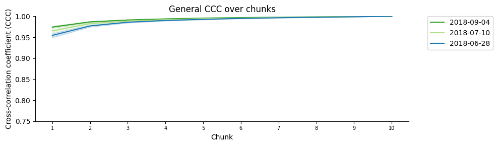
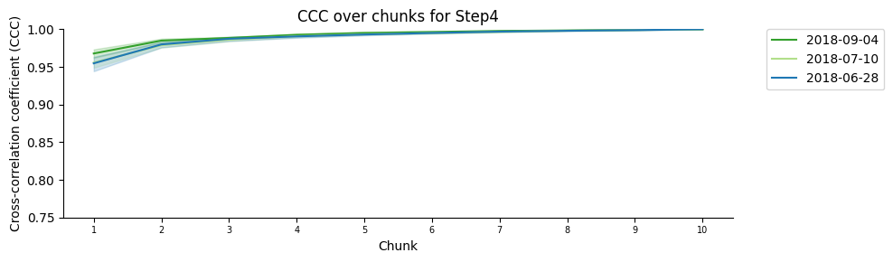
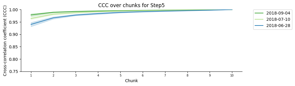
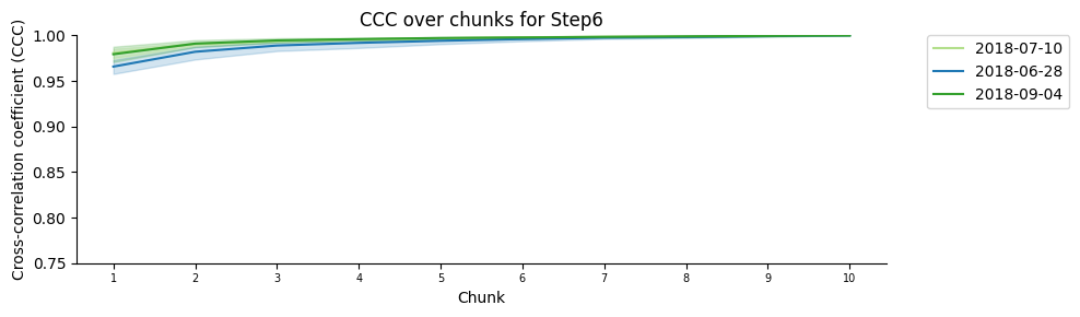
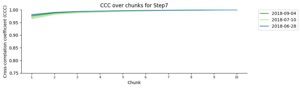
Assess by subsampling randomly over the time of aquisition to the final object (Saturation Plot)
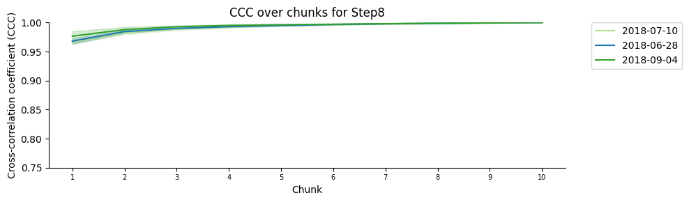
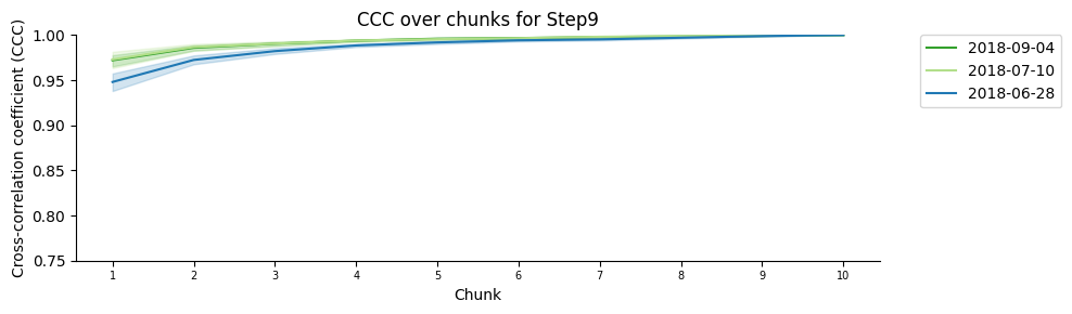
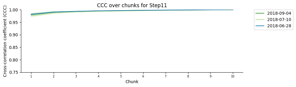
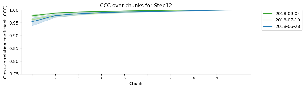
Here we will do a number of subgroups (chosen by the user) per timestep. For each timestep and subgroup, we will randomly assign ‘blinks’ from that timestep. Then we will compare that structure to the final structure with all the ‘blinks’ using a Cross Correlation Coefficient. Ideally we want that this CCC is high and stable through the different subsgroups.
Content:
Plot the mean saturation of the signal across the different steps.
Plot the mean saturation of the signal across the different walks.
Boxplot of the cross correlation coefficient across the different walks.
Create dataset for quality assessment by random subsamplig
if "dt_score_subsampling" not in globals() or not isinstance(dt_score_subsampling, pd.DataFrame):

    filename = f"quality_randomsubsampling{('_' + file_suffix) if file_suffix != '' else ''}.tsv"

    print("Trying to read pre-calculated quality with random subsampling from TSV file...")
    try:
        dt_score_subsampling = pd.read_csv(Path(tsv_folder, filename), sep='\t')

        if "flag" not in dt_score_subsampling.columns:
            dt_score_subsampling["flag"] = dt_score_subsampling[["experimentID","nucleusID","homolog","timepoint"]].astype(str).apply('_'.join, axis=1)

        print("Pre-calculated quality with random subsampling loaded from TSV file.")

    except FileNotFoundError:

        print("Pre-calculated TSV file not found. Calculating quality with random subsampling from scratch...")

        dt_score_subsampling = Batch_process_quality_assessment(obj_list = obj_list,
                                                    assessment_type = ["quality_randomsubsampling"],
                                                    library_n_Hype = number_of_steps_library+starting_step,
                                                    start_hype = starting_step,
                                                    prec_factor = 46,
                                                    metaInfo = ["experimentID","nucleusID","homolog"],
                                                    random_groups = number_of_random_groups)

        # This flag will help to identify unique walks
        dt_score_subsampling["flag"] = dt_score_subsampling[["experimentID","nucleusID","homolog","timepoint"]].astype(str).apply('_'.join, axis=1)
        dt_score_subsampling["Size"] = [info_df.loc[info_df["timepoint"] == ts, info_file_dict["column_size"]].values[0] for ts in dt_score_subsampling["timepoint"]]

        print("Saving quality with random subsampling to TSV file...", end="\r")
        dt_score_subsampling.drop(columns=["flag"]).to_csv(Path(tsv_folder, filename), sep='\t', index=False)
        print("Saving quality with random subsampling to TSV file... Done!")

        print("Quality with random subsampling calculated and saved to TSV file.")

    del filename

else:
    print("Quality with random subsampling DataFrame already exists in memory.")

if "cycle" in dt_score_subsampling.columns:

    dt_score_subsampling.rename(columns={"cycle": "chunk"}, inplace=True)

display(dt_score_subsampling.head(n=20))
Trying to read pre-calculated quality with random subsampling from TSV file...
Pre-calculated TSV file not found. Calculating quality with random subsampling from scratch...
Processing experimentID 2018-09-04, nucleusID 3, hom A (1/30).
Warning no segment 5 found
	Warning: missing segment 5 in experimentID 2018-09-04, nucleusID 3, hom A
Warning no segment 10 found
	Warning: missing segment 10 in experimentID 2018-09-04, nucleusID 3, hom A
Warning no segment 12 found
	Warning: missing segment 12 in experimentID 2018-09-04, nucleusID 3, hom A
Processing experimentID 2018-07-10, nucleusID 2, hom A (2/30).
Processing experimentID 2018-07-10, nucleusID 5, hom A (3/30).
Warning no segment 20 found
	Warning: missing segment 20 in experimentID 2018-07-10, nucleusID 5, hom A
Processing experimentID 2018-06-28, nucleusID 7, hom A (4/30).
Processing experimentID 2018-06-28, nucleusID 9, hom A (5/30).
Processing experimentID 2018-07-10, nucleusID 11, hom A (6/30).
Processing experimentID 2018-09-04, nucleusID 1, hom B (7/30).
Processing experimentID 2018-07-10, nucleusID 6, hom B (8/30).
Warning no segment 20 found
	Warning: missing segment 20 in experimentID 2018-07-10, nucleusID 6, hom B
Processing experimentID 2018-06-28, nucleusID 5, hom B (9/30).
Processing experimentID 2018-07-10, nucleusID 6, hom A (10/30).
Processing experimentID 2018-06-28, nucleusID 8, hom A (11/30).
Processing experimentID 2018-06-28, nucleusID 5, hom A (12/30).
Processing experimentID 2018-07-10, nucleusID 7, hom A (13/30).
Warning no segment 18 found
	Warning: missing segment 18 in experimentID 2018-07-10, nucleusID 7, hom A
Processing experimentID 2018-07-10, nucleusID 1, hom A (14/30).
Processing experimentID 2018-07-10, nucleusID 2, hom B (15/30).
Warning no segment 20 found
	Warning: missing segment 20 in experimentID 2018-07-10, nucleusID 2, hom B
Processing experimentID 2018-06-28, nucleusID 1, hom A (16/30).
Warning no segment 5 found
	Warning: missing segment 5 in experimentID 2018-06-28, nucleusID 1, hom A
Processing experimentID 2018-09-04, nucleusID 4, hom A (17/30).
Processing experimentID 2018-07-10, nucleusID 4, hom B (18/30).
Warning no segment 20 found
	Warning: missing segment 20 in experimentID 2018-07-10, nucleusID 4, hom B
Processing experimentID 2018-09-04, nucleusID 3, hom B (19/30).
Processing experimentID 2018-07-10, nucleusID 3, hom B (20/30).
Processing experimentID 2018-07-10, nucleusID 1, hom B (21/30).
Processing experimentID 2018-09-04, nucleusID 7, hom A (22/30).
Warning no segment 8 found
	Warning: missing segment 8 in experimentID 2018-09-04, nucleusID 7, hom A
Warning no segment 19 found
	Warning: missing segment 19 in experimentID 2018-09-04, nucleusID 7, hom A
Processing experimentID 2018-06-28, nucleusID 2, hom A (23/30).
Warning no segment 20 found
	Warning: missing segment 20 in experimentID 2018-06-28, nucleusID 2, hom A
Processing experimentID 2018-07-10, nucleusID 10, hom A (24/30).
Processing experimentID 2018-07-10, nucleusID 8, hom A (25/30).
Processing experimentID 2018-09-04, nucleusID 5, hom A (26/30).
Processing experimentID 2018-06-28, nucleusID 1, hom B (27/30).
Processing experimentID 2018-09-04, nucleusID 10, hom A (28/30).
Warning no segment 19 found
	Warning: missing segment 19 in experimentID 2018-09-04, nucleusID 10, hom A
Warning no segment 20 found
	Warning: missing segment 20 in experimentID 2018-09-04, nucleusID 10, hom A
Processing experimentID 2018-06-28, nucleusID 7, hom B (29/30).
Processing experimentID 2018-09-04, nucleusID 6, hom A (30/30).
Saving quality with random subsampling to TSV file... Done!
Quality with random subsampling calculated and saved to TSV file.
| experimentID | nucleusID | homolog | timepoint | name | chunk | ccc | nloc | assessment_type | flag | Size | |
|---|---|---|---|---|---|---|---|---|---|---|---|
| 0 | 2018-09-04 | 3 | A | 6 | Step2 | 1.0 | 0.993164 | 104.0 | quality_randomsubsampling | 2018-09-04_3_A_6 | 500 |
| 1 | 2018-09-04 | 3 | A | 6 | Step2 | 2.0 | 0.990234 | 195.0 | quality_randomsubsampling | 2018-09-04_3_A_6 | 500 |
| 2 | 2018-09-04 | 3 | A | 6 | Step2 | 3.0 | 0.995117 | 303.0 | quality_randomsubsampling | 2018-09-04_3_A_6 | 500 |
| 3 | 2018-09-04 | 3 | A | 6 | Step2 | 4.0 | 0.996094 | 411.0 | quality_randomsubsampling | 2018-09-04_3_A_6 | 500 |
| 4 | 2018-09-04 | 3 | A | 6 | Step2 | 5.0 | 0.996582 | 506.0 | quality_randomsubsampling | 2018-09-04_3_A_6 | 500 |
| 5 | 2018-09-04 | 3 | A | 6 | Step2 | 6.0 | 0.996582 | 609.0 | quality_randomsubsampling | 2018-09-04_3_A_6 | 500 |
| 6 | 2018-09-04 | 3 | A | 6 | Step2 | 7.0 | 0.997070 | 711.0 | quality_randomsubsampling | 2018-09-04_3_A_6 | 500 |
| 7 | 2018-09-04 | 3 | A | 6 | Step2 | 8.0 | 0.997559 | 802.0 | quality_randomsubsampling | 2018-09-04_3_A_6 | 500 |
| 8 | 2018-09-04 | 3 | A | 6 | Step2 | 9.0 | 0.999512 | 903.0 | quality_randomsubsampling | 2018-09-04_3_A_6 | 500 |
| 9 | 2018-09-04 | 3 | A | 6 | Step2 | 10.0 | 1.000000 | 990.0 | quality_randomsubsampling | 2018-09-04_3_A_6 | 500 |
| 10 | 2018-09-04 | 3 | A | 7 | Step3 | 1.0 | 0.975586 | 70.0 | quality_randomsubsampling | 2018-09-04_3_A_7 | 500 |
| 11 | 2018-09-04 | 3 | A | 7 | Step3 | 2.0 | 0.984863 | 132.0 | quality_randomsubsampling | 2018-09-04_3_A_7 | 500 |
| 12 | 2018-09-04 | 3 | A | 7 | Step3 | 3.0 | 0.988770 | 192.0 | quality_randomsubsampling | 2018-09-04_3_A_7 | 500 |
| 13 | 2018-09-04 | 3 | A | 7 | Step3 | 4.0 | 0.991699 | 273.0 | quality_randomsubsampling | 2018-09-04_3_A_7 | 500 |
| 14 | 2018-09-04 | 3 | A | 7 | Step3 | 5.0 | 0.992188 | 327.0 | quality_randomsubsampling | 2018-09-04_3_A_7 | 500 |
| 15 | 2018-09-04 | 3 | A | 7 | Step3 | 6.0 | 0.995117 | 389.0 | quality_randomsubsampling | 2018-09-04_3_A_7 | 500 |
| 16 | 2018-09-04 | 3 | A | 7 | Step3 | 7.0 | 0.995605 | 446.0 | quality_randomsubsampling | 2018-09-04_3_A_7 | 500 |
| 17 | 2018-09-04 | 3 | A | 7 | Step3 | 8.0 | 0.996582 | 508.0 | quality_randomsubsampling | 2018-09-04_3_A_7 | 500 |
| 18 | 2018-09-04 | 3 | A | 7 | Step3 | 9.0 | 0.997070 | 575.0 | quality_randomsubsampling | 2018-09-04_3_A_7 | 500 |
| 19 | 2018-09-04 | 3 | A | 7 | Step3 | 10.0 | 1.000000 | 645.0 | quality_randomsubsampling | 2018-09-04_3_A_7 | 500 |
Plot the mean saturation of the signal for each chromatin step
The different lines correspond to different walks.
Each walk is colored by date.
# General CCC over chunks plot
print("Plotting general CCC over chunks...")
plt.figure(figsize=(10, 3))
sns.lineplot(data=dt_score_subsampling,x='chunk',y='ccc',hue='experimentID',palette=color_palette)
plt.ylim(0.75,1.0)
plt.xlabel('Chunk')
plt.xticks(ticks=range(int(dt_score_subsampling['chunk'].min()), int(dt_score_subsampling['chunk'].max()) + 1), size = 7)
plt.ylabel('Cross-correlation coefficient (CCC)')
plt.title('General CCC over chunks')
plt.legend(bbox_to_anchor=(1.05, 1), loc=2, borderaxespad=0.)
sns.despine()
plt.tight_layout()
if save_plots:
filename = f"ccc_over_chunks{('_' + file_suffix) if file_suffix != '' else ''}.pdf"
plot_filename = Path(plots_folder, filename)
print(f"Saving plots to: {plot_filename}")
plt.savefig(plot_filename, **plot_opts)
del filename, plot_filename
else:
plt.show()
plt.close()
print(f"\n{'-'*54}\n")
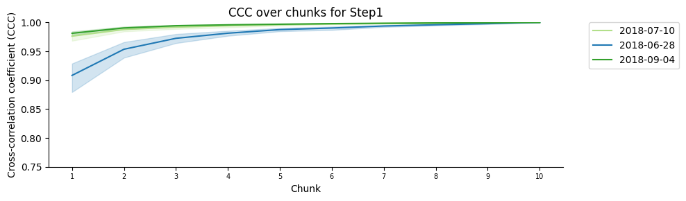
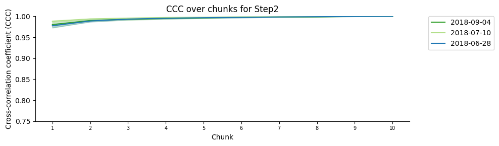
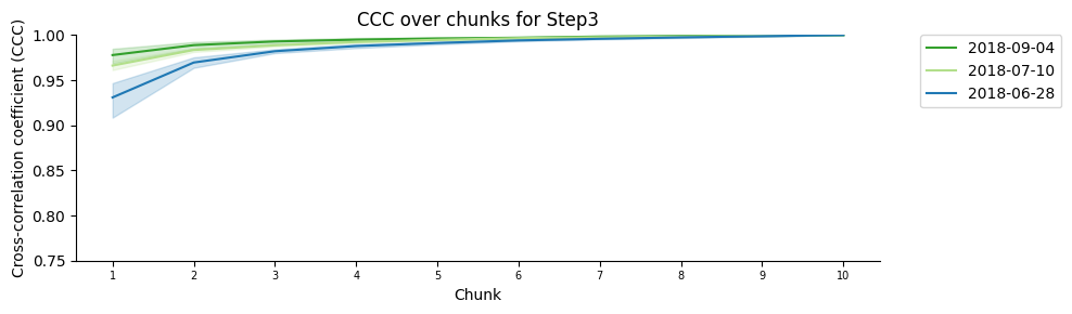
# CCC over chunks per timepoint plot
plot_per_step_folder = Path(plots_folder, "per_step")
plot_per_step_folder.mkdir(parents=True, exist_ok=True)
for i,g in dt_score_subsampling.groupby(["timepoint"]):
print (f"Plotting CCC of {tp_names[i[0]]} over chunks")
plt.figure(figsize=(10, 3))
sns.lineplot(data=g,x='chunk',y='ccc',hue='experimentID',palette=color_palette)
plt.ylim(0.75,1.0)
plt.xlabel('Chunk')
plt.xticks(ticks=range(int(g['chunk'].min()), int(g['chunk'].max()) + 1), size = 7)
plt.ylabel('Cross-correlation coefficient (CCC)')
plt.title(f'CCC over chunks for {tp_names[i[0]]}')
plt.legend(bbox_to_anchor=(1.05, 1), loc=2, borderaxespad=0.)
sns.despine()
plt.tight_layout()
if save_plots:
filename = f"ccc_over_chunk_step{i[0]}{('_' + file_suffix) if file_suffix != '' else ''}.pdf"
plot_filename = Path(plot_per_step_folder, filename)
print(f"Saving plots to: {plot_filename}")
plt.savefig(plot_filename, **plot_opts)
del filename, plot_filename
else:
plt.show()
plt.close()
print(f"\n{'-'*54}\n")
del i, g
Plotting general CCC over chunks...
------------------------------------------------------

Plotting CCC of Step1 over chunks
------------------------------------------------------

Plotting CCC of Step2 over chunks
------------------------------------------------------

Plotting CCC of Step3 over chunks
------------------------------------------------------

Plotting CCC of Step4 over chunks
------------------------------------------------------

Plotting CCC of Step5 over chunks
------------------------------------------------------

Plotting CCC of Step6 over chunks
------------------------------------------------------

Plotting CCC of Step7 over chunks
------------------------------------------------------

Plotting CCC of Step8 over chunks
------------------------------------------------------

Plotting CCC of Step9 over chunks
------------------------------------------------------

Plotting CCC of Step10 over chunks

------------------------------------------------------

Plotting CCC of Step11 over chunks
------------------------------------------------------

Plotting CCC of Step12 over chunks
------------------------------------------------------

Plotting CCC of Step13 over chunks
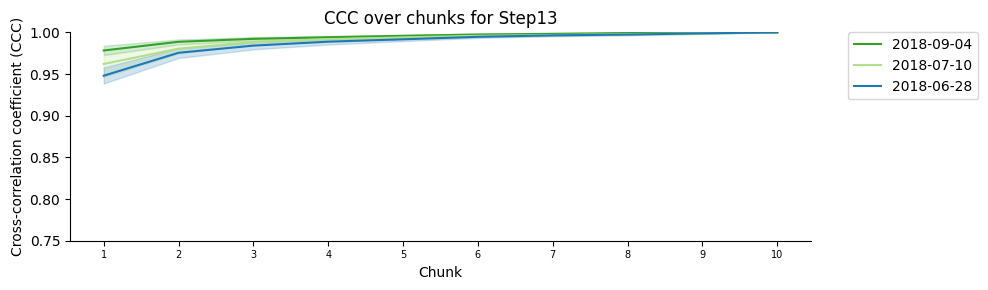
------------------------------------------------------

Plotting CCC of Step14 over chunks
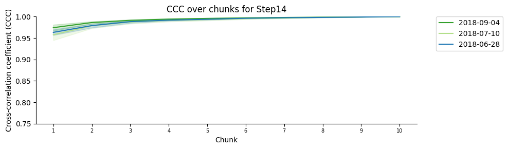
------------------------------------------------------

Plotting CCC of Step15 over chunks
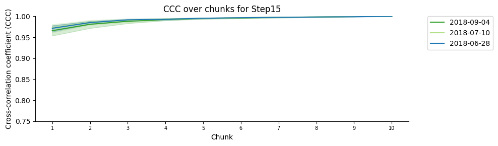
------------------------------------------------------

Plotting CCC of Step16 over chunks
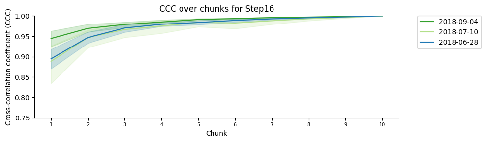
------------------------------------------------------
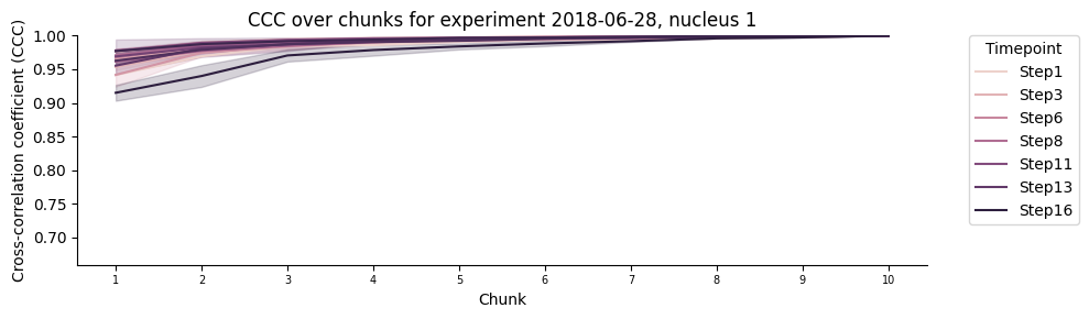
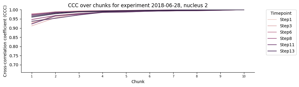
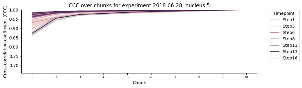
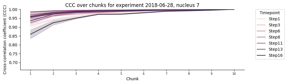
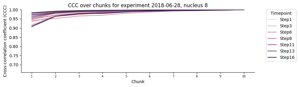
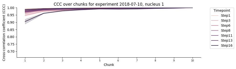
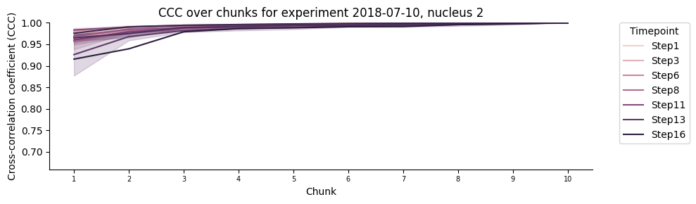
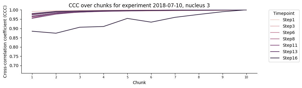
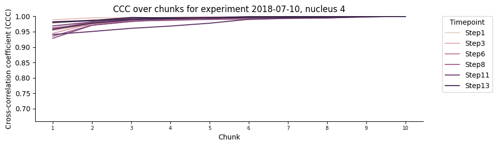
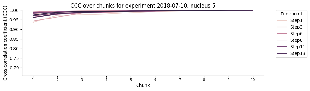
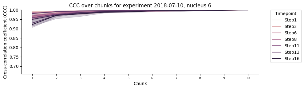
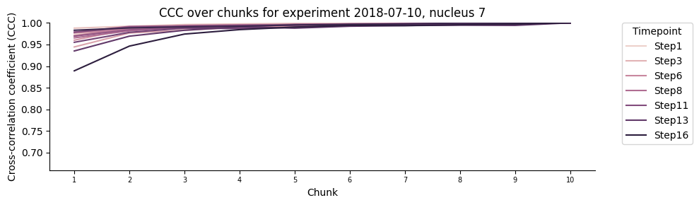
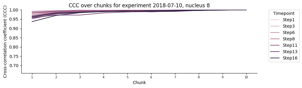
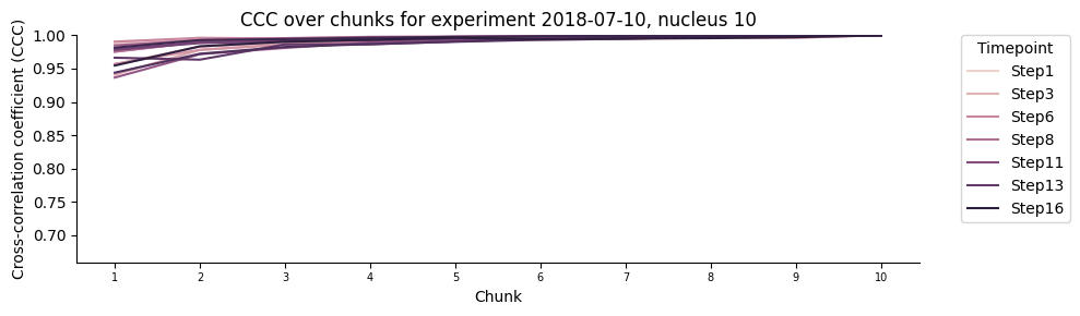
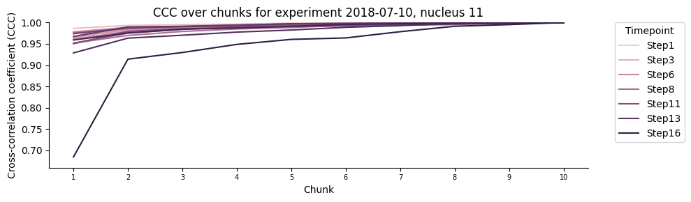
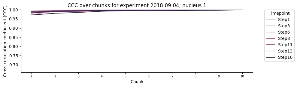
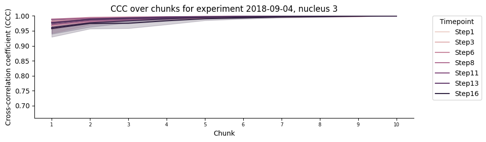
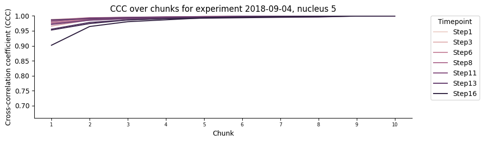
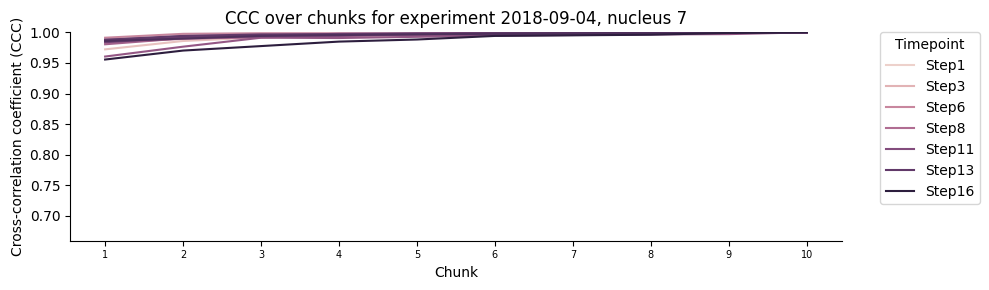
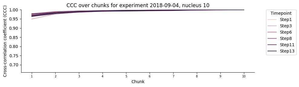
Plot the mean saturation of the signal for each walk
The different lines correspond to different chromatin steps.
plot_per_replica_folder = Path(plots_folder, "per_replica")
plot_per_replica_folder.mkdir(parents=True, exist_ok=True)

y_min = min(0.75, dt_score_subsampling['ccc'].min() - 0.025)

for (expID, nucleusID), g in dt_score_subsampling.groupby(["experimentID","nucleusID"]):
    print (f"Plotting CCC over chunks for experiment {expID}, nucleus {nucleusID}")

    plt.figure(figsize=(10, 3))

    sns.lineplot(data = g, x = 'chunk', y='ccc', hue = 'timepoint')

    plt.ylim(y_min,1.0)
    plt.xticks(ticks = range(int(g['chunk'].min()), int(g['chunk'].max()) + 1), size = 7)
    plt.xlabel('Chunk')
    plt.ylabel('Cross-correlation coefficient (CCC)')
    plt.title(f'CCC over chunks for experiment {expID}, nucleus {nucleusID}')
    plt.legend(bbox_to_anchor = (1.05, 1), loc = 2, borderaxespad = 0., title = 'Timepoint', labels = [tp_names[tp] if tp % 2 == 0 else None for tp in g['timepoint'].unique()])
    handles, labels = plt.gca().get_legend_handles_labels()
    labels = [tp_names[int(label)] for label in labels]
    keep = list(range(0, len(handles))) # Now shows 6 labels equally distributed. When can reduce further if needed.s
    plt.legend([handles[i] for i in keep], [labels[i] for i in keep],
               bbox_to_anchor=(1.05, 1), loc=2, borderaxespad=0., title='Timepoint')

    sns.despine()
    plt.tight_layout()

    if save_plots:
        filename = f"ccc_over_chunks_experiment_{expID}_nucleus_{nucleusID}{('_' + file_suffix) if file_suffix != '' else ''}.pdf"
        plot_filename = Path(plot_per_replica_folder, filename)
        print(f"Saving plots to: {plot_filename}")
        plt.savefig(plot_filename, **plot_opts)
        del filename, plot_filename
    else:
        plt.show()

    plt.close()

    print(f"\n{'-'*54}\n")

del expID, nucleusID, g, handles, labels, keep, plot_per_replica_folder, y_min
Plotting CCC over chunks for experiment 2018-06-28, nucleus 1
------------------------------------------------------

Plotting CCC over chunks for experiment 2018-06-28, nucleus 2
------------------------------------------------------

Plotting CCC over chunks for experiment 2018-06-28, nucleus 5
------------------------------------------------------

Plotting CCC over chunks for experiment 2018-06-28, nucleus 7
------------------------------------------------------

Plotting CCC over chunks for experiment 2018-06-28, nucleus 8
------------------------------------------------------

Plotting CCC over chunks for experiment 2018-06-28, nucleus 9

------------------------------------------------------

Plotting CCC over chunks for experiment 2018-07-10, nucleus 1
------------------------------------------------------

Plotting CCC over chunks for experiment 2018-07-10, nucleus 2
------------------------------------------------------

Plotting CCC over chunks for experiment 2018-07-10, nucleus 3
------------------------------------------------------

Plotting CCC over chunks for experiment 2018-07-10, nucleus 4
------------------------------------------------------

Plotting CCC over chunks for experiment 2018-07-10, nucleus 5
------------------------------------------------------

Plotting CCC over chunks for experiment 2018-07-10, nucleus 6
------------------------------------------------------

Plotting CCC over chunks for experiment 2018-07-10, nucleus 7
------------------------------------------------------

Plotting CCC over chunks for experiment 2018-07-10, nucleus 8
------------------------------------------------------

Plotting CCC over chunks for experiment 2018-07-10, nucleus 10
------------------------------------------------------

Plotting CCC over chunks for experiment 2018-07-10, nucleus 11
------------------------------------------------------

Plotting CCC over chunks for experiment 2018-09-04, nucleus 1
------------------------------------------------------

Plotting CCC over chunks for experiment 2018-09-04, nucleus 3
------------------------------------------------------

Plotting CCC over chunks for experiment 2018-09-04, nucleus 4

------------------------------------------------------

Plotting CCC over chunks for experiment 2018-09-04, nucleus 5
------------------------------------------------------

Plotting CCC over chunks for experiment 2018-09-04, nucleus 6

------------------------------------------------------

Plotting CCC over chunks for experiment 2018-09-04, nucleus 7
------------------------------------------------------

Plotting CCC over chunks for experiment 2018-09-04, nucleus 10
------------------------------------------------------
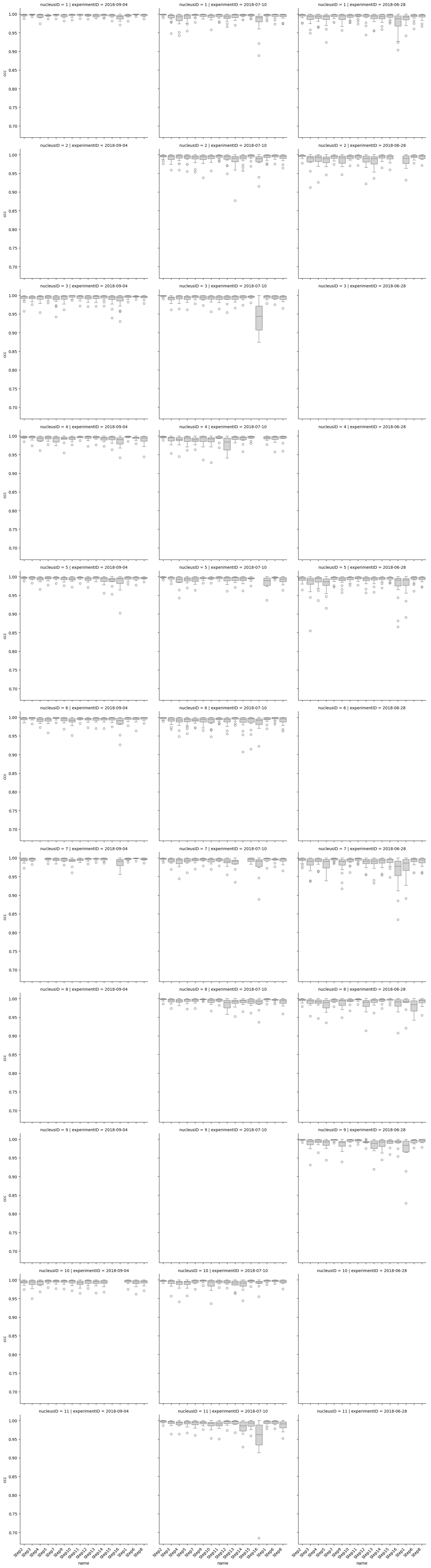
Boxplot of the CCC for each chromatin segments across all the walk
All in a single plot for an easier comparison.
g = sns.catplot(data=dt_score_subsampling, x="name", y="ccc", color="lightgrey",
            row="nucleusID", col="experimentID", kind='box', sharey = True)
for ax in g.axes.flat:
    ax.tick_params(axis='x', labelrotation=45)
    for label in ax.get_xticklabels():
        label.set_horizontalalignment('right')

sns.despine()
plt.tight_layout()

if save_plots:
    filename = f"ccc_boxplot_per_nucleus_and_experiment{('_' + file_suffix) if file_suffix != '' else ''}.pdf"
    plot_filename = Path(plots_folder, filename)
    print(f"Saving plots to: {plot_filename}")
    plt.savefig(plot_filename, **plot_opts)
    del filename, plot_filename
else:
    plt.show()

plt.close()

del g, ax, label
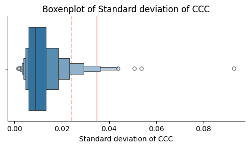
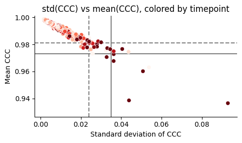
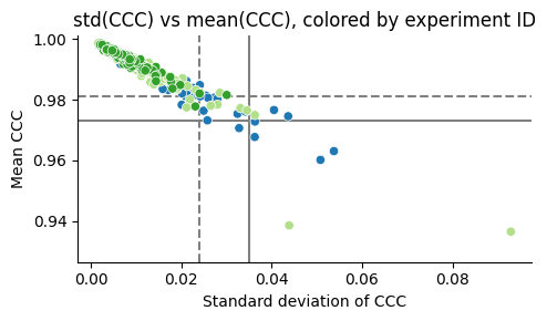
Generate summary table based on corralation variation of the quality assessment by random subsamplig aka “saturation plot”
Get summary of the CCC score and variation derived by the saturation plot.
High CCC score and smaller variation suggest that the chromatin segment (the 3D object) has been aquired stabily through time.
In the boxenplots for the mean, we selected those with a mean of CCC above the extreme/t1 outliers line (decided in the next cell).
In the boxenplots for the standard deviation, we selected those with a standard deviation of CCC below the extreme/mild outliers line (decided in the next cell).
saturation_plot_df = (dt_score_subsampling
    .groupby('flag')
    .agg(mean_CCC=('ccc', 'mean'),
         std_CCC =('ccc', 'std'),
         nloc     =('nloc', 'sum'))
)

t1_opts = {"color": "red", "alpha": 0.25, "zorder": 0, "linestyle": "--"}
t2_opts = {"color": "red", "alpha": 0.25, "zorder": 0, "linestyle": "-"}

# Here we will do a boxenplot of the mean CCC, and we will calculate the thresholds for outliers using the IQR method.
# We will also plot vertical lines for the thresholds of t1 and t2 outliers.
q1, q3 = saturation_plot_df["mean_CCC"].quantile([0.25, 0.75])
IQR = q3 - q1

t1_outliers_mean = (q1 - 1.5*IQR)
t2_outliers_mean = (q1 - 3.*IQR)

threshold_specs = [
    (t1_outliers_mean, t1_opts, "t1 outlier threshold"),
    (t2_outliers_mean, t2_opts, "t2 outlier threshold"),
]

print(f"Threshold for CCC mean of t1 outliers: {np.round(t1_outliers_mean, decimals = 3)}")
print(f"Using this threshold, we would expect {np.sum(saturation_plot_df['mean_CCC'] < t1_outliers_mean)} outliers in the mean CCC.\n")
print(f"Threshold for CCC mean of t2 outliers: {np.round(t2_outliers_mean, decimals = 3)}")
print(f"Using this threshold, we would expect {np.sum(saturation_plot_df['mean_CCC'] < t2_outliers_mean)} outliers in the mean CCC.\n")

_, ax = plt.subplots(figsize=(5, 3))
sns.boxenplot(data = saturation_plot_df, x = "mean_CCC", k_depth = "trustworthy", ax=ax)

for xval, opts, _ in threshold_specs:
    ax.axvline(x=xval, **opts)

ax.set(xlabel="Mean CCC", title="Boxenplot of Mean CCC")
sns.despine(ax=ax)
plt.tight_layout()

if save_plots:
    filename = f"boxenplot_mean_ccc{('_' + file_suffix) if file_suffix != '' else ''}.pdf"
    plot_filename = Path(plots_folder, filename)
    print(f"Saving plots to: {plot_filename}")
    plt.savefig(plot_filename, **plot_opts)
    del filename, plot_filename
else:
    plt.show()

plt.close()

print(f"\n{'-'*54}\n")

# Here we will do a boxenplot of the std CCC, and we will calculate the thresholds for outliers using the IQR method.
# We will also plot vertical lines for the thresholds of t1 and t2 outliers.
q1, q3 = saturation_plot_df["std_CCC"].quantile([0.25, 0.75])
IQR = q3 - q1

t1_outliers_std = (q3 + 1.5*IQR)
t2_outliers_std = (q3 + 3.*IQR)

threshold_specs = [
    (t1_outliers_std, t1_opts, "t1 outlier threshold"),
    (t2_outliers_std, t2_opts, "t2 outlier threshold"),
]

print(f"Threshold for CCC std of t1 outliers: {round(t1_outliers_std,3)}")
print(f"Using this threshold, we would expect {np.sum(saturation_plot_df['std_CCC'] > t1_outliers_std)} outliers in the std CCC.\n")
print(f"Threshold for CCC std of t2 outliers: {round(t2_outliers_std,3)}")
print(f"Using this threshold, we would expect {np.sum(saturation_plot_df['std_CCC'] > t2_outliers_std)} outliers in the std CCC.\n")

_, ax = plt.subplots(figsize=(5, 3))
sns.boxenplot(data=saturation_plot_df,x="std_CCC",k_depth="trustworthy", ax=ax)

for xval, opts, _ in threshold_specs:
    ax.axvline(x=xval, **opts)

ax.set(xlabel="Standard deviation of CCC", title="Boxenplot of Standard deviation of CCC")
sns.despine(ax=ax)
plt.tight_layout()

if save_plots:
    filename = f"boxenplot_std_ccc{('_' + file_suffix) if file_suffix != '' else ''}.pdf"
    plot_filename = Path(plots_folder, filename)
    print(f"Saving plots to: {plot_filename}")
    plt.savefig(plot_filename, **plot_opts)
    del filename, plot_filename
else:
    plt.show()

plt.close()

del t1_opts, t2_opts, q1, q3, IQR, threshold_specs, ax, opts, xval
Threshold for CCC mean of t1 outliers: 0.981
Using this threshold, we would expect 27 outliers in the mean CCC.

Threshold for CCC mean of t2 outliers: 0.973
Using this threshold, we would expect 7 outliers in the mean CCC.

------------------------------------------------------

Threshold for CCC std of t1 outliers: 0.024
Using this threshold, we would expect 27 outliers in the std CCC.

Threshold for CCC std of t2 outliers: 0.035
Using this threshold, we would expect 9 outliers in the std CCC.
saturation_plot_df = (dt_score_subsampling
    .groupby('flag')
    .agg(mean_CCC=('ccc', 'mean'),
         std_CCC =('ccc', 'std'),
         nloc     =('nloc', 'sum'))
)

saturation_plot_df['flag'] = saturation_plot_df.index
saturation_plot_df[["experimentID","nucleusID","homolog","timepoint"]] = saturation_plot_df['flag'].str.rsplit('_', expand=True)
saturation_plot_df["timepoint"] = pd.to_numeric(saturation_plot_df["timepoint"])
saturation_plot_df.reset_index(drop=True, inplace=True)

plt.figure(figsize=(5, 3))
sns.scatterplot(data=saturation_plot_df, x='std_CCC', y='mean_CCC', hue='timepoint', palette='Reds')
plt.ylim(np.nanmin([saturation_plot_df["mean_CCC"].min(), t2_outliers_mean]) - 0.01, 1.001)

plt.axvline(x=t1_outliers_std,  color="grey", zorder = 0, linestyle = "--")
plt.axhline(y=t1_outliers_mean, color="grey", zorder = 0, linestyle = "--")
plt.axvline(x=t2_outliers_std,  color="grey", zorder = 0, linestyle = "-")
plt.axhline(y=t2_outliers_mean, color="grey", zorder = 0, linestyle = "-")

plt.title('std(CCC) vs mean(CCC), colored by timepoint')
plt.xlabel('Standard deviation of CCC')
plt.ylabel('Mean CCC')
plt.legend([], [], frameon=False)

sns.despine()
plt.tight_layout()

if save_plots:
    filename = f"std_vs_mean_ccc_colored_by_timepoint{('_' + file_suffix) if file_suffix != '' else ''}.pdf"
    plot_filename = Path(plots_folder, filename)
    print(f"Saving plots to: {plot_filename}")
    plt.savefig(plot_filename, **plot_opts)
    del filename, plot_filename
else:
    plt.show()

plt.close()

print(f"\n{'-'*54}\n")

plt.figure(figsize=(5, 3))

sns.scatterplot(data=saturation_plot_df, x='std_CCC', y='mean_CCC', hue='experimentID',palette=color_palette)
plt.ylim(np.nanmin([saturation_plot_df["mean_CCC"].min(), t2_outliers_mean]) - 0.01, 1.001)

plt.axvline(x=t1_outliers_std,  color="grey", zorder = 0, linestyle = "--")
plt.axhline(y=t1_outliers_mean, color="grey", zorder = 0, linestyle = "--")
plt.axvline(x=t2_outliers_std,  color="grey", zorder = 0, linestyle = "-")
plt.axhline(y=t2_outliers_mean, color="grey", zorder = 0, linestyle = "-")

plt.title('std(CCC) vs mean(CCC), colored by experiment ID')
plt.legend([], [], frameon=False)
plt.xlabel('Standard deviation of CCC')
plt.ylabel('Mean CCC')
sns.despine()
plt.tight_layout()

if save_plots:
    filename = f"std_vs_mean_ccc_colored_by_experimentID{('_' + file_suffix) if file_suffix != '' else ''}.pdf"
    plot_filename = Path(plots_folder, filename)
    print(f"Saving plots to: {plot_filename}")
    plt.savefig(plot_filename, **plot_opts)
    del filename, plot_filename
else:
    plt.show()

plt.close()
------------------------------------------------------
Retrieve the list of tier1 and tier2 chromatin segment outliers (1.5xIQR (t1) and 3xIQR (Extreme_outliers), respectively) for which removal is strongly suggested.
cols2show = ["experimentID", "nucleusID", "homolog", "timepoint", "mean_CCC", "std_CCC"]

remove_t1_ccc = saturation_plot_df[(saturation_plot_df["mean_CCC"] <= t1_outliers_mean) |
                                   (saturation_plot_df["std_CCC"] >= t1_outliers_std)]

filename = Path(tsv_folder, f'segments2remove_bycccvariation_t1{("_" + file_suffix) if file_suffix != "" else ""}.tsv')
print(f"Saving t1 outlier segments to {filename}...", end = "\r")
remove_t1_ccc.drop(columns=["flag"]).to_csv(filename, sep='\t', index=False)
print(f"Saving t1 outlier segments to {filename}... Done!\n")

print(f"In case of using the t1 outliers, you should remove a total of {len(remove_t1_ccc)} out of {len(saturation_plot_df)} segments")
display(remove_t1_ccc[cols2show])

remove_t2_ccc = saturation_plot_df[(saturation_plot_df["mean_CCC"] <= t2_outliers_mean) |
                                   (saturation_plot_df["std_CCC"] >= t2_outliers_std)]

filename = Path(tsv_folder, f'segments2remove_bycccvariation_t2{("_" + file_suffix) if file_suffix != "" else ""}.tsv')
print(f"Saving t2 outlier segments to {filename}...", end = "\r")
remove_t2_ccc.drop(columns=["flag"]).to_csv(filename, sep="\t", index=False)
print(f"Saving t2 outlier segments to {filename}... Done!\n")

print(f"In case of using the t2 outliers, you should remove a total of {len(remove_t2_ccc)} out of {len(saturation_plot_df)} segments")
display(remove_t2_ccc[cols2show])

del t1_outliers_mean, t2_outliers_mean, t1_outliers_std, t2_outliers_std, cols2show, filename
Saving t1 outlier segments to /scratch/CIMA_tutorial/3_3D_reconstruction_assessment/tsvs/chr3/segments2remove_bycccvariation_t1_chr3.tsv... Done!

In case of using the t1 outliers, you should remove a total of 32 out of 466 segments
| experimentID | nucleusID | homolog | timepoint | mean_CCC | std_CCC | |
|---|---|---|---|---|---|---|
| 10 | 2018-06-28 | 1 | A | 20 | 0.970654 | 0.032810 |
| 38 | 2018-06-28 | 2 | A | 17 | 0.981152 | 0.020973 |
| 43 | 2018-06-28 | 2 | A | 7 | 0.980664 | 0.027305 |
| 56 | 2018-06-28 | 5 | A | 20 | 0.976611 | 0.040525 |
| 57 | 2018-06-28 | 5 | A | 5 | 0.975342 | 0.032443 |
| 61 | 2018-06-28 | 5 | A | 9 | 0.976367 | 0.024967 |
| 72 | 2018-06-28 | 5 | B | 20 | 0.972803 | 0.036308 |
| 75 | 2018-06-28 | 5 | B | 7 | 0.974561 | 0.043656 |
| 88 | 2018-06-28 | 7 | A | 20 | 0.960205 | 0.050801 |
| 89 | 2018-06-28 | 7 | A | 5 | 0.976074 | 0.034193 |
| 97 | 2018-06-28 | 7 | B | 13 | 0.981348 | 0.025468 |
| 104 | 2018-06-28 | 7 | B | 20 | 0.967725 | 0.036264 |
| 105 | 2018-06-28 | 7 | B | 5 | 0.973193 | 0.025793 |
| 110 | 2018-06-28 | 8 | A | 10 | 0.978320 | 0.020104 |
| 116 | 2018-06-28 | 8 | A | 16 | 0.980615 | 0.025913 |
| 120 | 2018-06-28 | 8 | A | 20 | 0.980371 | 0.028023 |
| 121 | 2018-06-28 | 8 | A | 5 | 0.984814 | 0.024125 |
| 133 | 2018-06-28 | 9 | A | 17 | 0.981104 | 0.024198 |
| 137 | 2018-06-28 | 9 | A | 5 | 0.963086 | 0.053775 |
| 166 | 2018-07-10 | 11 | A | 18 | 0.980029 | 0.021915 |
| 168 | 2018-07-10 | 11 | A | 20 | 0.936621 | 0.092926 |
| 184 | 2018-07-10 | 1 | A | 20 | 0.982422 | 0.024179 |
| 200 | 2018-07-10 | 1 | B | 20 | 0.977246 | 0.033098 |
| 213 | 2018-07-10 | 2 | A | 17 | 0.974951 | 0.036286 |
| 216 | 2018-07-10 | 2 | A | 20 | 0.978369 | 0.028040 |
| 247 | 2018-07-10 | 3 | B | 20 | 0.938672 | 0.043878 |
| 259 | 2018-07-10 | 4 | B | 16 | 0.977441 | 0.021204 |
| 291 | 2018-07-10 | 6 | A | 18 | 0.982275 | 0.028563 |
| 308 | 2018-07-10 | 6 | B | 19 | 0.978027 | 0.026534 |
| 323 | 2018-07-10 | 7 | A | 20 | 0.976465 | 0.034550 |
| 383 | 2018-09-04 | 3 | A | 20 | 0.977783 | 0.023116 |
| 430 | 2018-09-04 | 5 | A | 20 | 0.981543 | 0.030070 |
Saving t2 outlier segments to /scratch/CIMA_tutorial/3_3D_reconstruction_assessment/tsvs/chr3/segments2remove_bycccvariation_t2_chr3.tsv... Done!

In case of using the t2 outliers, you should remove a total of 10 out of 466 segments
| experimentID | nucleusID | homolog | timepoint | mean_CCC | std_CCC | |
|---|---|---|---|---|---|---|
| 10 | 2018-06-28 | 1 | A | 20 | 0.970654 | 0.032810 |
| 56 | 2018-06-28 | 5 | A | 20 | 0.976611 | 0.040525 |
| 72 | 2018-06-28 | 5 | B | 20 | 0.972803 | 0.036308 |
| 75 | 2018-06-28 | 5 | B | 7 | 0.974561 | 0.043656 |
| 88 | 2018-06-28 | 7 | A | 20 | 0.960205 | 0.050801 |
| 104 | 2018-06-28 | 7 | B | 20 | 0.967725 | 0.036264 |
| 137 | 2018-06-28 | 9 | A | 5 | 0.963086 | 0.053775 |
| 168 | 2018-07-10 | 11 | A | 20 | 0.936621 | 0.092926 |
| 213 | 2018-07-10 | 2 | A | 17 | 0.974951 | 0.036286 |
| 247 | 2018-07-10 | 3 | B | 20 | 0.938672 | 0.043878 |
Summary and filtering poorly assessed segments based on saturation plot
We recomend removing the T2 outliers at least. If you want to remove the T1 outliers (harsher filtering), modify the variale called threshold_precision to t1.
threshold_ccc = "t2"

if threshold_ccc == "t1":
    if "remove_t1_ccc" in locals() and remove_t1_ccc is not None:
        remove_ccc = remove_t1_ccc.copy() if not remove_t1_ccc.empty else pd.DataFrame()
    else:
        filename = Path(tsv_folder, f'segments2remove_bycccvariation_t1{("_" + file_suffix) if file_suffix != "" else ""}.tsv')
        remove_ccc = pd.read_table(filename, sep="\t")
        del filename
elif threshold_ccc == "t2":
    if "remove_t2_ccc" in locals() and remove_t2_ccc is not None:
        remove_ccc = remove_t2_ccc.copy() if not remove_t2_ccc.empty else pd.DataFrame()
    else:
        filename = Path(tsv_folder, f'segments2remove_bycccvariation_t2{("_" + file_suffix) if file_suffix != "" else ""}.tsv')
        remove_ccc = pd.read_table(filename, sep="\t")
        del filename
else:
    print("Invalid threshold_ccc value. Please choose 't1' or 't2'.")

if not remove_ccc.empty:
    remove_ccc["flag"] = remove_ccc[["experimentID","nucleusID","homolog","timepoint"]].astype(str).apply('_'.join, axis=1)
    flag_segment_toremove = remove_ccc.flag.unique()
    dt_filtered = saturation_plot_df[(~saturation_plot_df['flag'].isin(flag_segment_toremove))]

    print(f"A total of {len(saturation_plot_df)- len(dt_filtered)} out of {len(saturation_plot_df)} segments were removed after applying the {threshold_ccc} outlier threshold.")
    del flag_segment_toremove
else:
    dt_filtered = saturation_plot_df.copy()
    print(f"No segments to remove based on the selected threshold for CCC.")
A total of 10 out of 466 segments were removed after applying the t2 outlier threshold.
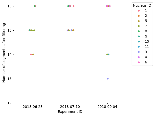
Should we take this plots out and just leave the efficiency plot at the end?
dt_stats = dt_filtered.groupby(["experimentID","nucleusID","homolog"]).size().reset_index(name='timepoints_count')

sns.stripplot(data = dt_stats, x = "experimentID", y = "timepoints_count", jitter = True, hue = "nucleusID")

plt.legend(title = "Nucleus ID", bbox_to_anchor = (1.05, 1), loc = 2, borderaxespad = 0.)
plt.yticks(ticks = range(int(dt_stats['timepoints_count'].min()) - 1, int(dt_stats['timepoints_count'].max()) + 1, 1))
plt.ylabel('Number of segments after filtering')
plt.xlabel('Experiment ID')
sns.despine()
plt.tight_layout()

if save_plots:
    filename = f"stripplot_experiment_vs_counts_after_filtering{('_' + file_suffix) if file_suffix != '' else ''}.pdf"
    plot_filename = Path(plots_folder, filename)
    print(f"Saving plots to: {plot_filename}")
    plt.savefig(plot_filename, **plot_opts)
    del filename, plot_filename
else:
    plt.show()

plt.close()
number_of_nucleus = 0
number_of_diploids = 0
number_of_not_diploid = 0
full_walk_counter = 0
partial_walk_count = 0

for _, g in dt_stats.groupby(["experimentID","nucleusID"]):
    number_of_nucleus += 1

    if g.shape[0] != 2:
        number_of_not_diploid += 1
        continue

    number_of_diploids += 1

    c0, c1 = g.timepoints_count.tolist()

    if c0 != c1:
        partial_walk_count+=1
    else:
        full_walk_counter+=1

number_of_fully_walked_homologs=0
number_of_homologs=0
fully_walked_homologs_id=[]

for i,g in dt_stats.groupby(["experimentID","nucleusID","homolog"]):
    number_of_homologs += 1
    if g.timepoints_count.item()==number_of_steps_library:
        number_of_fully_walked_homologs += 1
        fully_walked_homologs_id.append(i)

print(f"Number of nuclei acquired: {number_of_nucleus}\n")
print(f"Number of diploid nuclei: {number_of_diploids}")
print(f"\tFully walked (both copies are present): {full_walk_counter}\n")
print(f"Number of homologs: {number_of_homologs}")
print(f"\tFully walked: {number_of_fully_walked_homologs}")

del number_of_nucleus, number_of_diploids, number_of_not_diploid, full_walk_counter, partial_walk_count, g, i
del number_of_fully_walked_homologs, fully_walked_homologs_id
if 'c0' in locals():
    del c0
if 'c1' in locals():
    del c1
Number of nuclei acquired: 23

Number of diploid nuclei: 7
	Fully walked (both copies are present): 3

Number of homologs: 30
	Fully walked: 12
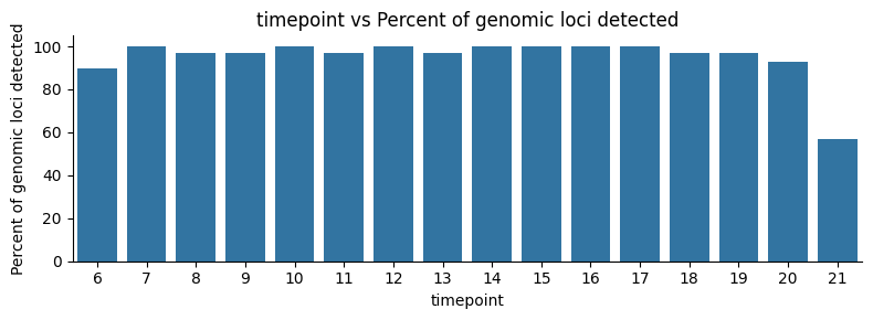
Here we check the percentage of steps detected after filtering the walks according to the thresholds set before. We also repeat one of the earlier plots to see the difference.
stats_timepoint=dt_filtered.groupby(["timepoint"]).size().reset_index(name='counts')
stats_timepoint['Percent'] = round((stats_timepoint.counts)*100/number_of_homologs)
stats_timepoint = stats_timepoint.merge(info_df, left_on = "timepoint", right_on = "timepoint")
display(stats_timepoint)
plt.figure(figsize=(8,3))
sns.barplot(x="timepoint",y="Percent",data=stats_timepoint)
plt.xlabel('timepoint')
plt.xticks(ticks=list(range(0, len(stats_timepoint))), labels=stats_timepoint['timepoint']+1)
plt.ylabel('Percent of genomic loci detected')
plt.title('timepoint vs Percent of genomic loci detected')
sns.despine()
plt.tight_layout()
if save_plots:
filename = f"barplot_timepoint_vs_percent_filtered{('_' + file_suffix) if file_suffix != '' else ''}.pdf"
plot_filename = Path(plots_folder, filename)
print(f"Saving plots to: {plot_filename}")
plt.savefig(plot_filename, **plot_opts)
del filename, plot_filename
else:
plt.show()
plt.close()
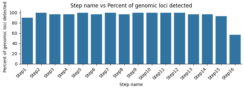
plt.figure(figsize=(8,3))
sns.barplot(x="Name",y="Percent",data=stats_timepoint)
plt.xticks(rotation=45, ha="right")
plt.xlabel('Step name')
plt.ylabel('Percent of genomic loci detected')
plt.title('Step name vs Percent of genomic loci detected')
sns.despine()
plt.tight_layout()
if save_plots:
filename = f"barplot_name_vs_percent_filtered{('_' + file_suffix) if file_suffix != '' else ''}.pdf"
plot_filename = Path(plots_folder, filename)
print(f"Saving plots to: {plot_filename}")
plt.savefig(plot_filename, **plot_opts)
del filename, plot_filename
else:
plt.show()
plt.close()
del stats_timepoint, number_of_homologs
| timepoint | counts | Percent | Round | Chr | Start(hg19) | End(hg19) | Name | Size(kb) | |
|---|---|---|---|---|---|---|---|---|---|
| 0 | 5 | 27 | 90.0 | 6 | chr3 | 150000000 | 150500000 | Step1 | 500 |
| 1 | 6 | 30 | 100.0 | 7 | chr3 | 150500000 | 151000000 | Step2 | 500 |
| 2 | 7 | 29 | 97.0 | 8 | chr3 | 151000000 | 151500000 | Step3 | 500 |
| 3 | 8 | 29 | 97.0 | 9 | chr3 | 151500000 | 152000000 | Step4 | 500 |
| 4 | 9 | 30 | 100.0 | 10 | chr3 | 152000000 | 152500000 | Step5 | 500 |
| 5 | 10 | 29 | 97.0 | 11 | chr3 | 152500000 | 153000000 | Step6 | 500 |
| 6 | 11 | 30 | 100.0 | 12 | chr3 | 153000000 | 153500000 | Step7 | 500 |
| 7 | 12 | 29 | 97.0 | 13 | chr3 | 153500000 | 154000000 | Step8 | 500 |
| 8 | 13 | 30 | 100.0 | 14 | chr3 | 154000000 | 154500000 | Step9 | 500 |
| 9 | 14 | 30 | 100.0 | 15 | chr3 | 154500000 | 155000000 | Step10 | 500 |
| 10 | 15 | 30 | 100.0 | 16 | chr3 | 155000000 | 155500000 | Step11 | 500 |
| 11 | 16 | 30 | 100.0 | 17 | chr3 | 155500000 | 156000000 | Step12 | 500 |
| 12 | 17 | 29 | 97.0 | 18 | chr3 | 156000000 | 156500000 | Step13 | 500 |
| 13 | 18 | 29 | 97.0 | 19 | chr3 | 156500000 | 157000000 | Step14 | 500 |
| 14 | 19 | 28 | 93.0 | 20 | chr3 | 157000000 | 157500000 | Step15 | 500 |
| 15 | 20 | 17 | 57.0 | 21 | chr3 | 157500000 | 158000000 | Step16 | 500 |
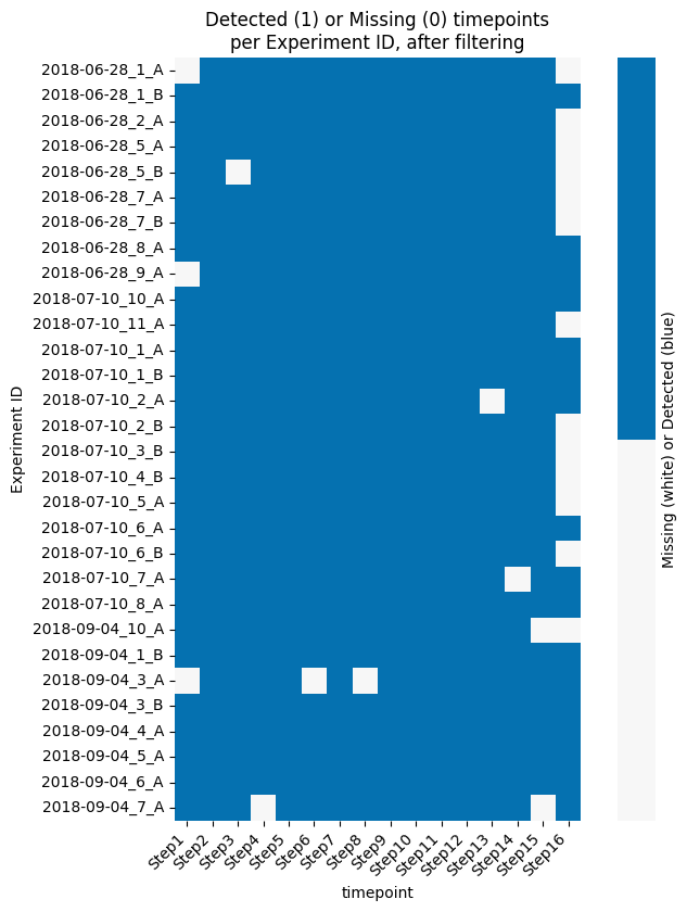
# Add flag column for each walk
dt_filtered.loc[:, "flag"] = dt_filtered[["experimentID", "nucleusID", "homolog"]].astype(str).apply('_'.join, axis=1)
# Count unique timepoints per walk
df_count = (dt_filtered.groupby("flag")["timepoint"].nunique().reset_index(name="timepoint_count"))
# Create stats DataFrame: one row per (flag, timepoint)
dt_stats = (dt_filtered[["experimentID", "nucleusID", "homolog", "flag", "timepoint"]].drop_duplicates().assign(bool=1))
# Plot a heatmap of the timepoints for each unique ID with a color bar indicating "Detected" (1) or "missing" (0)
mx = dt_stats.pivot(index='flag', columns='timepoint', values='bool').fillna(0).astype(int)
# Check that we have all the timepoints present in info_df in mx, if not, add 0s
for tp in info_df["timepoint"]:
if tp not in mx.columns:
mx[tp] = 0
# Reorder the columns of mx to match the order in info_df
mx = mx[sorted(mx.columns, key=lambda x: info_df[info_df["timepoint"] == x].index[0])]
# Dynamically adjust figure size for large datasets
fig_width = min(1 + 0.4 * mx.shape[1], 20)
fig_height = min(1 + 0.25 * mx.shape[0], 20)
# Heatmap that shows detected (1) or missing (0) timepoints
plt.figure(figsize=(fig_width, fig_height))
sns.heatmap(data = mx, square=True, cmap=['#f7f7f7', '#0571b0'], vmin=0, vmax=1,
cbar_kws={'label': 'Missing (white) or Detected (blue)', 'ticks': []})
plt.xlabel('timepoint')
plt.xticks(ticks=[i + 0.5 for i in range(mx.shape[1])], labels=[tp_names[tp] for tp in mx.columns], rotation=45, ha='right')
plt.ylabel('Experiment ID')
plt.title('Detected (1) or Missing (0) timepoints\nper Experiment ID, after filtering')
sns.despine(top = True, right = True, bottom = True, left = True)
plt.tight_layout()
if save_plots:
filename = f"detected_missing_timepoints_heatmap_filtered{('_' + file_suffix) if file_suffix != '' else ''}.pdf"
plot_filename = Path(plots_folder, filename)
print(f"Saving plots to: {plot_filename}")
plt.savefig(plot_filename, **plot_opts)
del filename, plot_filename
else:
plt.show()
plt.close()
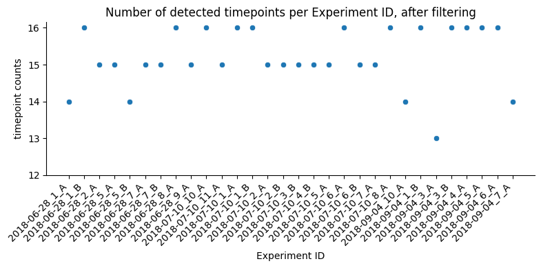
# Scatter plot of the number of timepoints for each unique ID
plt.figure(figsize=(np.ceil(len(df_count) / 4), 4))
sns.scatterplot(data=df_count, x="flag", y="timepoint_count")
plt.xticks(rotation=45, ha='right')
plt.yticks(range(int(df_count['timepoint_count'].min()) - 1, int(df_count['timepoint_count'].max()) + 1, 1))
plt.xlabel("Experiment ID")
plt.ylabel("timepoint counts")
plt.title("Number of detected timepoints per Experiment ID, after filtering")
sns.despine()
plt.tight_layout()
if save_plots:
filename = f"number_of_detected_timepoints_per_experimentID_filtered{('_' + file_suffix) if file_suffix != '' else ''}.pdf"
plot_filename = Path(plots_folder, filename)
print(f"Saving plots to: {plot_filename}")
plt.savefig(plot_filename, **plot_opts)
del filename, plot_filename
else:
plt.show()
plt.close()
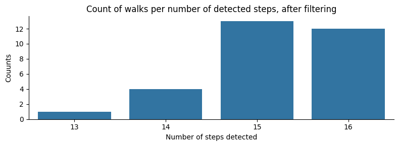
# Plot with the count of the number of walks for every timepoint size
plt.figure(figsize=(8, 3))
sns.countplot(df_count, x="timepoint_count")
plt.xlabel("Number of steps detected")
plt.ylabel("Couunts")
plt.title("Count of walks per number of detected steps, after filtering")
sns.despine()
plt.tight_layout()
if save_plots:
filename = f"count_of_walks_per_number_of_detected_steps_filtered{('_' + file_suffix) if file_suffix != '' else ''}.pdf"
plot_filename = Path(plots_folder, filename)
print(f"Saving plots to: {plot_filename}")
plt.savefig(plot_filename, **plot_opts)
del filename, plot_filename
else:
plt.show()
plt.close()
del df_count, mx, fig_width, fig_height, tp
# Get a list of all CSV files in the specified data folder
csv_files = list(data_folder.glob('*.csv'))

if len(csv_files) == 0:
    print("No files found, please input the correct work_folder")
else:
    print(f"Total number of files found: {len(csv_files)}")

print("Loading the experimental quality data from the CSV files")
traces_pass = pd.read_csv(Path(experimental_assessment_folder, f"experimental_assessment_pass_{file_suffix}.txt"), sep="\t", names=["trace"])

# Get a list of metadata keys to extract from filenames
metadata_keys = ["nucleusID", "cellID", "locationID", "date", "homolog", "chromosome"]

# Initialize an empty list to store the StructuralObject instances
obj_list = []

rownames = []

if len(csv_files) > 0:
    # Iterate over each file in the list of file names
    efficiency_matrix_3 = np.zeros((len(csv_files), number_of_steps_library))
    for count, filein in enumerate(csv_files, start=1):

        stem = Path(filein).stem

        print(f"Processing file {count}: {stem}")

        # We mine the metadata from the filename using regex patterns. If not possible, assign default values.
        metadata_CIMA = {
            key: (match.group(1) if (match := regex_patterns[key].search(stem)) else default)
            for key, default in zip(metadata_keys, [count, count, count, stem, "A", "chrN"])
        }

        # Adjust the metadata for nucleus and cell (if nucleus is count, but cell is something, use the cell match in nucleus)
        if "cell" in metadata_CIMA and metadata_CIMA["nucleusID"] == count:
            metadata_CIMA["nucleusID"] = metadata_CIMA["cell"]

        metadata_CIMA["nucleusID"] = int(metadata_CIMA["nucleusID"])
        metadata_CIMA["cellID"] = int(metadata_CIMA["cellID"])
        metadata_CIMA["locationID"] = int(metadata_CIMA["locationID"])

        # Set experimentID as date for consistency
        metadata_CIMA["experimentID"] = metadata_CIMA["date"]

        # Read the CSV file and create a StructuralObject instance
        objin = CSVParser.read_CSV_file(filein.as_posix(), metadata = metadata_CIMA, content_type = "srx")

        # Filter the atomList to include only the specified timepoints in the info file
        objin.atomList = objin.atomList[(objin.atomList['timepoint'] >= starting_step - 1) &
                                        (objin.atomList['timepoint'] < (starting_step + number_of_steps_library - 1))].copy()

        rownames.append(f"{objin.metadata['experimentID']}_cell{objin.metadata['nucleusID']}_{objin.metadata['homolog']}")

        if not stem in traces_pass["trace"].values:
            print(f"\tSkipping file {count}: {stem} because it did not pass the experimental quality assessment.")
            continue

        for tp in objin.atomList['timepoint'].unique():
            temp = dt_filtered[(dt_filtered["experimentID"] == metadata_CIMA["experimentID"]) &
                               (dt_filtered["nucleusID"] == str(metadata_CIMA["nucleusID"])) &
                               (dt_filtered["homolog"] == metadata_CIMA["homolog"]) &
                               (dt_filtered["timepoint"] == tp)]

            if not temp.empty:
                efficiency_matrix_3[count-1, tp-starting_step] = 1

efficiency_matrix_3 = pd.DataFrame(efficiency_matrix_3, columns=tp_names.values())
efficiency_matrix_3.index = rownames

del csv_files, traces_pass, metadata_keys, rownames, count, filein, stem, metadata_CIMA, objin, tp, temp, match
Total number of files found: 33
Loading the experimental quality data from the CSV files
Processing file 1: 2018-09-04_nuc03_A_chr3
Processing file 2: 2018-07-10_nuc04_A_chr3
	Skipping file 2: 2018-07-10_nuc04_A_chr3 because it did not pass the experimental quality assessment.
Processing file 3: 2018-07-10_nuc02_A_chr3
Processing file 4: 2018-07-10_nuc05_A_chr3
Processing file 5: 2018-07-10_nuc03_A_chr3
	Skipping file 5: 2018-07-10_nuc03_A_chr3 because it did not pass the experimental quality assessment.
Processing file 6: 2018-06-28_nuc07_A_chr3
Processing file 7: 2018-06-28_nuc09_A_chr3
Processing file 8: 2018-07-10_nuc11_A_chr3
Processing file 9: 2018-09-04_nuc01_B_chr3
Processing file 10: 2018-07-10_nuc06_B_chr3
Processing file 11: 2018-06-28_nuc05_B_chr3
Processing file 12: 2018-07-10_nuc06_A_chr3
Processing file 13: 2018-06-28_nuc08_A_chr3
Processing file 14: 2018-06-28_nuc05_A_chr3
Processing file 15: 2018-07-10_nuc07_A_chr3
Processing file 16: 2018-07-10_nuc01_A_chr3
Processing file 17: 2018-07-10_nuc02_B_chr3
Processing file 18: 2018-06-28_nuc01_A_chr3
Processing file 19: 2018-09-04_nuc04_A_chr3
Processing file 20: 2018-07-10_nuc04_B_chr3
Processing file 21: 2018-09-04_nuc03_B_chr3
Processing file 22: 2018-07-10_nuc03_B_chr3
Processing file 23: 2018-07-10_nuc01_B_chr3
Processing file 24: 2018-09-04_nuc07_A_chr3
Processing file 25: 2018-06-28_nuc02_A_chr3
Processing file 26: 2018-09-04_nuc01_A_chr3
	Skipping file 26: 2018-09-04_nuc01_A_chr3 because it did not pass the experimental quality assessment.
Processing file 27: 2018-07-10_nuc10_A_chr3
Processing file 28: 2018-07-10_nuc08_A_chr3
Processing file 29: 2018-09-04_nuc05_A_chr3
Processing file 30: 2018-06-28_nuc01_B_chr3
Processing file 31: 2018-09-04_nuc10_A_chr3
Processing file 32: 2018-06-28_nuc07_B_chr3
Processing file 33: 2018-09-04_nuc06_A_chr3
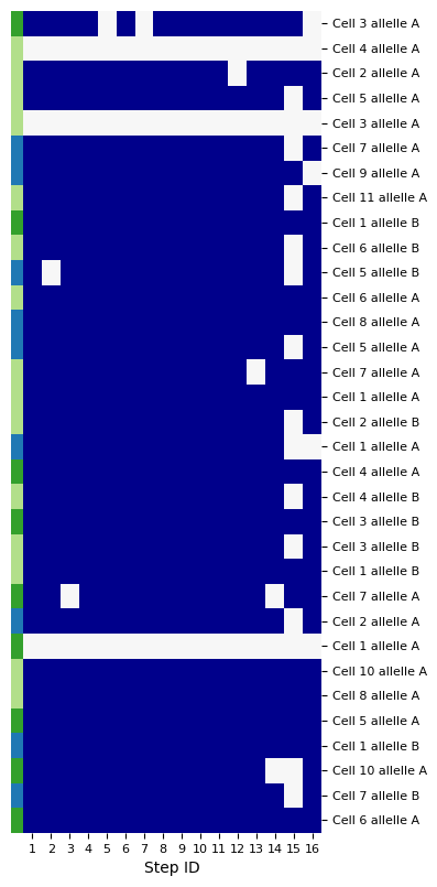
rownames = [f"Cell {temp.split('_')[1].replace('cell', '')} allelle {temp.split('_')[2]}" for temp in efficiency_matrix_3.index]

fig_height = max(2, 0.3 * len(efficiency_matrix_3.index))

g = sns.clustermap(data = efficiency_matrix_3,
               cmap=['#f7f7f7', '#00008B'],
               vmin=0, vmax=1,
               figsize=(5, fig_height),
               row_colors=[color_palette.get(d.split("_")[0], "#a6cee3") for d in efficiency_matrix_3.index],
               col_cluster=False,
               row_cluster=False,
               yticklabels=rownames,
               xticklabels=[f"{i+1}" for i in range(efficiency_matrix_3.shape[1])],
               method='average',
               metric='euclidean',
)
g.ax_heatmap.set_xlabel('Step ID')
g.ax_heatmap.set_xticklabels(g.ax_heatmap.get_xticklabels(), rotation=0, fontsize=8)
g.ax_heatmap.set_yticklabels(g.ax_heatmap.get_yticklabels(), rotation=0, fontsize=8)
g.ax_row_dendrogram.set_visible(False)
g.ax_col_dendrogram.set_visible(False)
g.ax_cbar.set_visible(False)

if save_plots:
    filename = f"efficiency_matrix_post_reconstruction_assessment{('_' + file_suffix) if file_suffix != '' else ''}.pdf"
    plot_filename = Path(plots_folder, filename)
    print(f"Saving plots to: {plot_filename}")
    plt.savefig(plot_filename, **plot_opts)
    del filename, plot_filename
else:
    plt.show()
plt.close()

del g, rownames
Show the different walks that we have
If you want to see them, uncomment the lines (take out the # that is at the start of every line)
# from CIMA.segments.SegmentGaussian import TransformBlurrer as TB
# from CIMA.utils.Visualization import plot3DMultipleMapsMarchingCubes

# import warnings
# # This line is to filter out a UserWarning that is raised when doing the plot. Then we re-enable the warnings.
# warnings.filterwarnings("ignore", category=UserWarning)

# for experimentID, nucleus, homolog in fully_walked_homologs_id:
#     for obj in obj_list:
#         if obj.metadata["experimentID"]==experimentID and \
#            obj.metadata["nucleusID"]==nucleus and \
#            obj.metadata["homolog"]==homolog :
#             # print (obj)

#             listobj=obj.split_into_time()
#             listobj_map=[TB.SR_gaussian_blur(segment = i, resolution=45, sigma_coeff=1) for i in listobj.values()]

#             print(f"Plotting 3D maps for experiment {experimentID}, nucleus {nucleus}, homolog {homolog}")
#             fig=plot3DMultipleMapsMarchingCubes(listobj_map, labels=listobj.keys(), scalars=listobj.keys(),cmap="Blues")
#             fig.show()
#             fig.close()

# warnings.filterwarnings("default", category=UserWarning)
print()