1 - Guided identification of chromatin segments
Description: This notebook contains an example pipeline to read SRX localization data (in csv format) and perform clustering detection of genomic loci.
CIMA offers two density-based cluster analysis options: (i) Density-based spatial clustering of applications with noise (DBSCAN) (ii) Density-Based Clustering Based on Hierarchical Density Estimates (HDBSCAN)
In this example pipeline we will use DBSCAN option. DBSCAN relies on two parameters:
‘eps’ is the maximum distance between two data points to be considered in the same neighborhood
It defines the neighborhood around a data point i.e. if the distance between two points is lower or equal to ‘eps’ then they are considered as neighbors. If the eps value is chosen too small then a large part of the data will be considered as noise. If it is chosen very large then the clusters will merge and majority of the data points will be in the same clusters. In CIMA the optimal eps value is chosen based on the k-distance graph that allows for an estimate of the noise level versus signal.
‘min_samples’ is the minimum amount of neighbors a data points should have signal
Minimum number of neighbors (data points) within eps radius. The denser the dataset, the larger value of min_samples must be chosen. As a general rule, the minimum min_samples can be derived from the number of dimensions D in the dataset as, MinPts >= D+1. The minimum value of MinPts must be chosen at least 3.
We will get back to this in the dedicated section of the notebook.
The notebooks provide an example of varied steps in the pipelines that the user can perform. Note, density based methods are heavily biased by the presence of beads in the FOV/ROI. Altough we implemented a function to remove them from drift-corrected point-clouds, we raccomend the user to take care of them before running this pipeline.
Content:
Read file and create a structural object in the chromatin universe
Filter localization by varied evaluators from structural object
Detect beads in the FOV
Define a user-defined ROI
Detection of genomic regions with DBSCAN grid sreach
Batch-process
Next notebook to run is:
Experimental quality assessment
#import libaries
import os
import matplotlib.pyplot as plt
import seaborn as sns

from cima.segments.segment_info import *
from cima.parsers.parser_csv import *
from cima.utils.visualization import *
from cima.detection import clusters as CL
from cima.detection import beads_identification as BI
from cima.segments import segment_gaussian as SG
Read file and create a structural object in the chromatin universe
# Define the input path and file name
pathin = "TEST/"
filein = "SVABext027_MS-rep_loc003_co16_bg50_xy20-z40_cell3_nb_r124_dc1.csv"

# Read the CSV file and create a structural object in the chromatin universe
# The content_type specifies which content should be required from the file (srx, thunderstorm, xyztimepoint, free) and how the columns should be ranamed
# The metadata dictionary contains additional information about the experiment
# - "experimentID": A unique identifier for the experiment
# - "date": The date when the experiment was conducted
# - in can recive user-define metadata
objIN = CSVParser.read_CSV_file(pathin + filein, metadata={"experimentID": "test", "date": "19_04"},content_type="srx")
print(objIN)
Filename: TEST/SVABext027_MS-rep_loc003_co16_bg50_xy20-z40_cell3_nb_r124_dc1.csv
No Of Localisation: 730223
First Localisation:(Time 0  ClusterID 0 Chromosome 0: 27095.8 ,14800.9 ,-439.851)
Last Localisation: (Time 3  ClusterID 0 Chromosome 0: 43553.4 ,9042.31 ,3342.33)
# Print the metadata of the structural object
print(objIN.metadata)
{'experimentID': 'test', 'date': '19_04', 'filename': 'TEST/SVABext027_MS-rep_loc003_co16_bg50_xy20-z40_cell3_nb_r124_dc1.csv'}
#Metadatinfo
objIN.metadata
{'experimentID': 'test',
 'date': '19_04',
 'filename': 'TEST/SVABext027_MS-rep_loc003_co16_bg50_xy20-z40_cell3_nb_r124_dc1.csv'}
The core of a Segment object is its atomList attribute, which contains a pandas DataFrame with all the data about localizations
objIN.atomList.columns
Index(['imageID', 'cycle', 'zstep', 'frame', 'accum', 'photoncount',
       'photoncount11', 'photoncount12', 'photoncount21', 'photoncount22',
       'psfx', 'psfy', 'psfz', 'psfphotoncount', 'x', 'y', 'z', 'amp',
       'background11', 'background12', 'background21', 'background22',
       'maxResidualSlope', 'chi', 'loglike', 'accuracy', 'llr', 'timepoint',
       'xprec', 'yprec', 'zprec', 'frame-timestamp', 'vis-probe',
       'record_name', 'clusterID', 'chromosomes', 's11', 's12', 'shiftz',
       'mass'],
      dtype='object')
To determine the number of time steps are forming a givven structural object, we use the no_of_Times() method in CIMA. This method returns the number of distinct time steps present in the structural object,.
nSteps=objIN.no_of_Times()
print ("no_of_Times:",nSteps)
no_of_Times: 3
# Get a single time segment from the structural object

obj = objIN.get_Time_segment(timepoint=1)

# Alternative: one can get multiple time segments using the get_multiple_Time_segment method
# obj_multiple = obj.get_multiple_Time_segment(timepoints=[1, 2, 3])
Filter localization by varied evaluators from structural object
Precision Filter
The PrecisionFilter method is used to filter localizations based on their precision values. Precision values are typically associated with the uncertainty in the localization of points in the dataset. By applying this filter, we can remove points that have high uncertainty, thereby improving the quality of the data for further analysis.
The factor parameter is a list that specifies the threshold for filtering in each dimension (x, y, z). In this example, factor=[20,20,50] means that localizations with precision values greater than 50 in any of the x, y, or z dimensions will be filtered out.
obj=obj.PrecisionFilter(factor=[50,50,50])
print (obj)
Filename: TEST/SVABext027_MS-rep_loc003_co16_bg50_xy20-z40_cell3_nb_r124_dc1.csv
No Of Localisation: 293159
First Localisation:(Time 1  ClusterID 0 Chromosome 0: 26565.4 ,16846.0 ,-300.668)
Last Localisation: (Time 1  ClusterID 0 Chromosome 0: 35727.2 ,13044.3 ,3402.43)
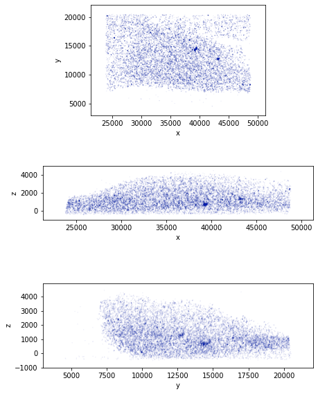
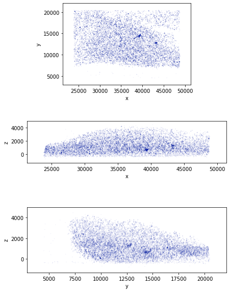
To visualize the point cloud data in 2D, we use the CIMA plotClustering2DProjections function to plot the 2D projections of the subsampled coordinates. To speed up the plotting we create a random subsample of the coordinates with approximately 10% of the points from the full dataset.
coord=obj.Getcoord()
sub=coord[np.random.choice([True, False], len(coord), replace=True, p=[0.1, 0.9])]
fig=plotClustering2DProjections(sub)
fig.show()
/var/folders/xq/7zsdfhq12yq1gq3789_q_3hr0000gn/T/ipykernel_31505/2629043428.py:4: UserWarning: Matplotlib is currently using module://matplotlib_inline.backend_inline, which is a non-GUI backend, so cannot show the figure.
  fig.show()
coord
array([[26565.4  , 16846.   ,  -300.668],
       [29210.4  , 16926.5  ,   379.981],
       [47235.4  ,  9174.81 ,   345.697],
       ...,
       [33757.8  ,  9411.71 ,  3553.89 ],
       [33782.9  ,  9414.26 ,  3561.47 ],
       [35727.2  , 13044.3  ,  3402.43 ]])
We can also visualize the point cloud in 3D with the CIMA plotClustering3D function
fig=plotClustering3D(sub,point_size=0.1)
fig.show()
Precision Filter
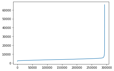
To visualize the distribution of photon counts, we can use a line plot. The following code sorts the photon counts and then plots them using Seaborn’s lineplot function.
Note, by accessing the atomList object one can filter the data based on teh arameters of choice.
sns.lineplot(np.sort(obj.atomList.psfphotoncount))
plt.show()
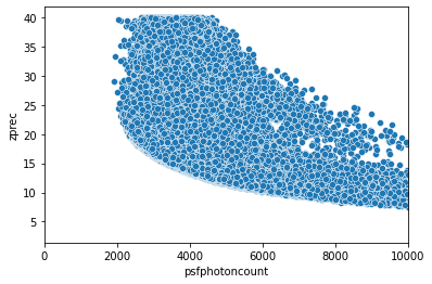
We suggest to plot Z precision as function of photon count to aid filtering of localisation
sns.scatterplot(x=obj.atomList.psfphotoncount,y=obj.atomList.zprec)
plt.xlim(0, 10000)
(0.0, 10000.0)
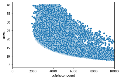
If you are working with a FOV we suggest to filter by photon count to reduce the noise level.
The PhotonCount_Filter method is used to filter localizations based on their photon count values. This helps in removing localizations that have photon counts outside a specified range, thereby reducing noise and improving the quality of the data.
In the following code, we apply the PhotonCount_Filter method with an upperbound_factor of 35000 and a lowerbound_factor of 2000. This means that localizations with photon counts outside this range will be filtered out. We also applied another filter to include only those localizations where the z precision (zprec) is greater than or equal to 5.
The goal here is to filter out localisation belonging to beads.
# Apply Photon Count Filter
# The PhotonCount_Filter method is used to filter localizations based on their photon count values.
# This helps in removing localizations that have photon counts outside a specified range, thereby reducing noise and improving the quality of the data.
# In the following code, we apply the PhotonCount_Filter method with an upperbound_factor of 35000 and a lowerbound_factor of 2000.
# This means that localizations with photon counts outside this range will be filtered out.
obj_filtered = obj.PhotonCount_Filter(upperbound_factor=35000, lowerbound_factor=100)

# Further filter the data based on z precision
# Here, we filter the atomList to include only those localizations where the z precision (zprec) is greater than or equal to 5.
objtmp = obj_filtered.atomList[(obj_filtered.atomList.zprec >= 5)]

# Create a new Segment object with the filtered content
# The copyWithNewContent method creates a new Segment object using the filtered atomList.
obj_filtered = obj_filtered.copyWithNewContent(objtmp)
print (obj_filtered)
Filename: TEST/SVABext027_MS-rep_loc003_co16_bg50_xy20-z40_cell3_nb_r124_dc1.csv
No Of Localisation: 293132
First Localisation:(Time 1  ClusterID 0 Chromosome 0: 26565.4 ,16846.0 ,-300.668)
Last Localisation: (Time 1  ClusterID 0 Chromosome 0: 35727.2 ,13044.3 ,3402.43)
sns.scatterplot(x=obj_filtered.atomList.psfphotoncount,y=obj_filtered.atomList.zprec)
plt.xlim(0, 10000)
(0.0, 10000.0)
coord=obj_filtered.Getcoord()
sub=coord[np.random.choice([True, False], len(coord), replace=True, p=[0.1, 0.9])]
fig=plotClustering2DProjections(sub)
fig.show()
/var/folders/xq/7zsdfhq12yq1gq3789_q_3hr0000gn/T/ipykernel_31505/1686059948.py:4: UserWarning: Matplotlib is currently using module://matplotlib_inline.backend_inline, which is a non-GUI backend, so cannot show the figure.
  fig.show()
If needed the user can select a ROI to reduce the computational time. Here we show how to manually selected a ROI. In thsi example case the file is already a ROI selected so the entire object is set as the ROI.
# #obj_filtered
# objtmp=obj_filtered.atomList[(obj_filtered.atomList.x>=12000) & (obj_filtered.atomList.x<=16500)\
#                                     & (obj_filtered.atomList.y<=16000) & (obj_filtered.atomList.y>=7000)\
#                                     & (obj_filtered.atomList.z<=3500) & (obj_filtered.atomList.z>0) ]
# obj_ROI=obj_filtered.copyWithNewContent(objtmp)
obj_ROI=obj_filtered
coord=obj_ROI.Getcoord()
fig=plotClustering3D(coord,point_size=0.1)
fig.show()
Detection of genomic regions with DBSCAN grid sreach
With CIMA you can identify imaged chromatin segments inside the point-cloud. Moreover, as we will see in the following notebooks, CIMA also allows to compute a set of morphological and spatial features about the identified clusters.
Here we show one of the approaches used for the identification of clusters, based on the DBSCAN algorithm.
This clustering algorithm classifies as signal (as opposed to noise) all those localizations with an estimated density around them lower than a specific threshold. It then groups in a cluster all those signal-localizations which are respectively “reachable”.
The estimation of density and the definitions of the threshold and of reachability, all depend on two parameters: eps and min_pts.
To select the right pair of parameters we use the principle of stability: the best parameters are the ones that give you most similar results if you change them slightly. To find the best ones according to this approach we perform a grid search over a set of candidates.
The selection of parameters and the running of DBSCAN is all included in the class DBscan_grid_search_stable. However before applying that, we want to visualize something that is also included in the class, but which also gives us some insights about the experiment: the definition of eps candidates.
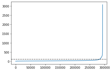
Indeed it’s interesting to visualize how the distance to the k-th neighbor increases when we sort them. The distance at which we see the plot suddenly pointing upwards (meaning that the localization sparsity increases) is a good starting point for the eps parameter.
eps=CL.searchepsilon(obj_ROI.Getcoord(),show=True)
eps=(round(eps))
print (eps)
113
To segment the localized and drift-corrected point cloud data within each ROI into chromatin signal or as noise component we implement a semi-automatic procedure based on a hyperparamenter search of DSBCAN to identified the optimal parameter pairs.
# Initialize the DBSCAN grid search object
scanner=CL.DBscan_grid_search_stable()


# Fit the DBSCAN grid search to the ROI object
# Parameters:
# - obj_ROI: The region of interest segment object to be clustered
# - consider_noise: Whether to consider noise points in the clustering labels returned (True means noise points will be considered)
# - n_neighbors: The number to set the kth-proximal neighbors to use when estimating the ARI score (2 in this case).
# - conv: Whether to use convergence criteria for the grid search (True means the search will stop early if convergence is detected)
# - verbose: The verbosity level of the output (2 means detailed output will be printed)
# - n_jobs: The number of parallel jobs to run (8 means 8 parallel jobs will be used)
# - downsampling_rate: The rate at which to uniformly downsample the data (1.0 means no downsampling) this can be used to speed up the calcualtion and to derive a conversion factor.
# - random_seed: The seed for the random number generator (0 means the results will be reproducible)
# - limit_density: Whether to limit parameter-space density, set to True it will detect a pairs of parameters  between the 25th and 75th percentiles of the distribution of estimated density among all points in the dataset.
scanner.fit(obj_ROI, consider_noise=True, n_neighbors=2,
            conv=True, verbose=2, n_jobs=8, downsampling_rate=1., random_seed=0,limit_density=True)
searching epsilon
self.min_pts_range:  [ 10  20  30  40  50  60  70  80  90 100 110 120 130 140 150 160 170 180
 190 200 220 230 240 250 260 270 300 350 400]
self.eps_range:  [ 50  55  61  67  73  79  85  91  97 103 109 115 121 127 133 139 144 150
 156 162]
10  -  50
10  -  55
10  -  61
10  -  67
10  -  73
10  -  79
10  -  85
10  -  91
10  -  97
10  -  103
10  -  109
10  -  115
10  -  121
10  -  127
10  -  133
10  -  139
10  -  144
10  -  150
10  -  156
10  -  162
20  -  50mputation:  3.4 %
20  -  55
20  -  61
20  -  67
20  -  73
20  -  79
20  -  85
20  -  91
20  -  97
20  -  103
20  -  109
20  -  115
20  -  121
20  -  127
20  -  133
20  -  139
20  -  144
20  -  150
20  -  156
20  -  162
30  -  50mputation:  6.9 %
30  -  55
30  -  61
30  -  67
30  -  73
30  -  79
30  -  85
30  -  91
30  -  97
30  -  103
30  -  109
30  -  115
30  -  121
30  -  127
30  -  133
30  -  139
30  -  144
30  -  150
30  -  156
30  -  162
40  -  50mputation:  10.3 %
40  -  55
40  -  61
40  -  67
40  -  73
40  -  79
40  -  85
40  -  91
40  -  97
40  -  103
40  -  109
40  -  115
40  -  121
40  -  127
40  -  133
40  -  139
40  -  144
40  -  150
40  -  156
40  -  162
50  -  50mputation:  13.8 %
50  -  55
50  -  61
50  -  67
50  -  73
50  -  79
50  -  85
50  -  91
50  -  97
50  -  103
50  -  109
50  -  115
50  -  121
50  -  127
50  -  133
50  -  139
50  -  144
50  -  150
50  -  156
50  -  162
60  -  50mputation:  17.2 %
60  -  55
60  -  61
60  -  67
60  -  73
60  -  79
60  -  85
60  -  91
60  -  97
60  -  103
60  -  109
60  -  115
60  -  121
60  -  127
60  -  133
60  -  139
60  -  144
60  -  150
60  -  156
60  -  162
70  -  50mputation:  20.7 %
70  -  55
70  -  61
70  -  67
70  -  73
70  -  79
70  -  85
70  -  91
70  -  97
70  -  103
70  -  109
70  -  115
70  -  121
70  -  127
70  -  133
70  -  139
70  -  144
70  -  150
70  -  156
70  -  162
80  -  50mputation:  24.1 %
80  -  55
80  -  61
80  -  67
80  -  73
80  -  79
80  -  85
80  -  91
80  -  97
80  -  103
80  -  109
80  -  115
80  -  121
80  -  127
80  -  133
80  -  139
80  -  144
80  -  150
80  -  156
80  -  162
90  -  50mputation:  27.6 %
90  -  55
90  -  61
90  -  67
90  -  73
90  -  79
90  -  85
90  -  91
90  -  97
90  -  103
90  -  109
90  -  115
90  -  121
90  -  127
90  -  133
90  -  139
90  -  144
90  -  150
90  -  156
90  -  162
100  -  50putation:  31.0 %
100  -  55
100  -  61
100  -  67
100  -  73
100  -  79
100  -  85
100  -  91
100  -  97
100  -  103
100  -  109
100  -  115
100  -  121
100  -  127
100  -  133
100  -  139
100  -  144
100  -  150
100  -  156
100  -  162
110  -  50putation:  34.5 %
110  -  55
110  -  61
110  -  67
110  -  73
110  -  79
110  -  85
110  -  91
110  -  97
110  -  103
110  -  109
110  -  115
110  -  121
110  -  127
110  -  133
110  -  139
110  -  144
110  -  150
110  -  156
110  -  162
120  -  50putation:  37.9 %
120  -  55
120  -  61
120  -  67
120  -  73
120  -  79
120  -  85
120  -  91
120  -  97
120  -  103
120  -  109
120  -  115
120  -  121
120  -  127
120  -  133
120  -  139
120  -  144
120  -  150
120  -  156
120  -  162
130  -  50putation:  41.4 %
130  -  55
130  -  61
130  -  67
130  -  73
130  -  79
130  -  85
130  -  91
130  -  97
130  -  103
130  -  109
130  -  115
130  -  121
130  -  127
130  -  133
130  -  139
130  -  144
130  -  150
130  -  156
130  -  162
140  -  50putation:  44.8 %
140  -  55
140  -  61
140  -  67
140  -  73
140  -  79
140  -  85
140  -  91
140  -  97
140  -  103
140  -  109
140  -  115
140  -  121
140  -  127
140  -  133
140  -  139
140  -  144
140  -  150
140  -  156
140  -  162
150  -  50putation:  48.3 %
150  -  55
150  -  61
150  -  67
150  -  73
150  -  79
150  -  85
150  -  91
150  -  97
150  -  103
150  -  109
150  -  115
150  -  121
150  -  127
150  -  133
150  -  139
150  -  144
150  -  150
150  -  156
150  -  162
160  -  50putation:  51.7 %
160  -  55
160  -  61
160  -  67
160  -  73
160  -  79
160  -  85
160  -  91
160  -  97
160  -  103
160  -  109
160  -  115
160  -  121
160  -  127
160  -  133
160  -  139
160  -  144
160  -  150
160  -  156
160  -  162
170  -  50putation:  55.2 %
170  -  55
170  -  61
170  -  67
170  -  73
170  -  79
170  -  85
170  -  91
170  -  97
170  -  103
170  -  109
170  -  115
170  -  121
170  -  127
170  -  133
170  -  139
170  -  144
170  -  150
170  -  156
170  -  162
180  -  50putation:  58.6 %
180  -  55
180  -  61
180  -  67
180  -  73
180  -  79
180  -  85
180  -  91
180  -  97
180  -  103
180  -  109
180  -  115
180  -  121
180  -  127
180  -  133
180  -  139
180  -  144
180  -  150
180  -  156
180  -  162
190  -  50putation:  62.1 %
190  -  55
190  -  61
190  -  67
190  -  73
190  -  79
190  -  85
190  -  91
190  -  97
190  -  103
190  -  109
190  -  115
190  -  121
190  -  127
190  -  133
190  -  139
190  -  144
190  -  150
190  -  156
190  -  162
200  -  50putation:  65.5 %
200  -  55
200  -  61
200  -  67
200  -  73
200  -  79
200  -  85
200  -  91
200  -  97
200  -  103
200  -  109
200  -  115
200  -  121
200  -  127
200  -  133
200  -  139
200  -  144
200  -  150
200  -  156
200  -  162
220  -  50putation:  69.0 %
220  -  55
220  -  61
220  -  67
220  -  73
220  -  79
220  -  85
220  -  91
220  -  97
220  -  103
220  -  109
220  -  115
220  -  121
220  -  127
220  -  133
220  -  139
220  -  144
220  -  150
220  -  156
220  -  162
230  -  50putation:  72.4 %
230  -  55
230  -  61
230  -  67
230  -  73
230  -  79
230  -  85
230  -  91
230  -  97
230  -  103
230  -  109
230  -  115
230  -  121
230  -  127
230  -  133
230  -  139
230  -  144
230  -  150
230  -  156
230  -  162
240  -  50putation:  75.9 %
240  -  55
240  -  61
240  -  67
240  -  73
240  -  79
240  -  85
240  -  91
240  -  97
240  -  103
240  -  109
240  -  115
240  -  121
240  -  127
240  -  133
240  -  139
240  -  144
240  -  150
240  -  156
240  -  162
250  -  50putation:  79.3 %
250  -  55
250  -  61
250  -  67
250  -  73
250  -  79
250  -  85
250  -  91
250  -  97
250  -  103
250  -  109
250  -  115
250  -  121
250  -  127
250  -  133
250  -  139
250  -  144
250  -  150
250  -  156
250  -  162
260  -  50putation:  82.8 %
260  -  55
260  -  61
260  -  67
260  -  73
260  -  79
260  -  85
260  -  91
260  -  97
260  -  103
260  -  109
260  -  115
260  -  121
260  -  127
260  -  133
260  -  139
260  -  144
260  -  150
260  -  156
260  -  162
270  -  50putation:  86.2 %
270  -  55
270  -  61
270  -  67
270  -  73
270  -  79
270  -  85
270  -  91
270  -  97
270  -  103
270  -  109
270  -  115
270  -  121
270  -  127
270  -  133
270  -  139
270  -  144
270  -  150
270  -  156
270  -  162
300  -  50putation:  89.7 %
300  -  55
300  -  61
300  -  67
300  -  73
300  -  79
300  -  85
300  -  91
300  -  97
300  -  103
300  -  109
300  -  115
300  -  121
300  -  127
300  -  133
300  -  139
300  -  144
300  -  150
300  -  156
300  -  162
350  -  50putation:  93.1 %
350  -  55
350  -  61
350  -  67
350  -  73
350  -  79
350  -  85
350  -  91
350  -  97
350  -  103
350  -  109
350  -  115
350  -  121
350  -  127
350  -  133
350  -  139
350  -  144
350  -  150
350  -  156
350  -  162
400  -  50putation:  96.6 %
400  -  55
400  -  61
400  -  67
400  -  73
400  -  79
400  -  85
400  -  91
400  -  97
400  -  103
400  -  109
400  -  115
400  -  121
400  -  127
400  -  133
400  -  139
400  -  144
400  -  150
400  -  156
400  -  162
dbscan computation:  100.0 %
Starting min_points: 28 out of 29
<CIMA.detection.clusters.DBscan_grid_search_stable at 0x7fc3bf72c070>
Note, if needed one can extend the grid search without having to recompute the labels with the mergeOtherDBSCANGrid fucntion
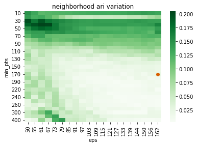
Plot the grid-search to see which combination of parameters was selected as the one to use for the clustering.
The selected ones are those that achieved the highest neighborhood similiary and the smallest neighborhood variation.
scanner.plotAriGrid()
plt.show()
scanner.plotAriVarGrid()
plt.show()
scanner.saveLog("TEST/DBSCAN_gridsearch.csv")
scattering at: [19.5, 16.5]

scattering at: [19.5, 16.5]
Get labels for the optimal combination of parameters
scanner.labels_
array([-1, -1, -1, ..., -1, -1, -1])
Define the clustered structural object retrived with the optimal combination of parameters and plot it
objout=scanner.optimal_segment


coord=objout.Getcoord()
fig=plotClustering2DProjections(coord,scanner.labels_)
fig.show()
/var/folders/xq/7zsdfhq12yq1gq3789_q_3hr0000gn/T/ipykernel_31505/2342635911.py:6: UserWarning: Matplotlib is currently using module://matplotlib_inline.backend_inline, which is a non-GUI backend, so cannot show the figure.
  fig.show()
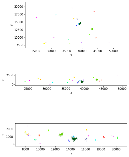
list(set(scanner.labels_))
[0, 1, 2, 3, 4, 5, 6, 7, 8, 9, 10, 11, 12, 13, 14, 15, 16, 17, 18, 19, -1]
fig=plotClustering3D(coord,scanner.labels_,show_noise=False,point_size=1)
fig.show()
#
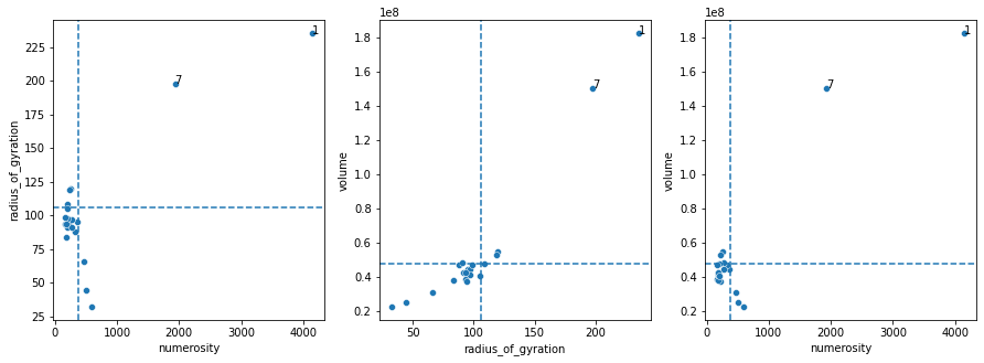
As shown in the previouse plot, varied clusters are detected. CIMA implements a strategy to distinguish chromatin segments clusters from non-specific signals
, based on varied parameters. We suggest to use a combination of number of localisations (numerosity), volume, and radius of gyration.
The ThresholdClusterFilter class provides this functionality. Here we show it based on proportion to teh maximal cluster.
selection = CL.ThresholdClusterFilter()
selection.fit(objout,features_to_use = ['radius_of_gyration', 'volume','numerosity'], method='percentile', n_jobs=8)
selection.plot(label_clusters=True)
getSegmentsFeatures: computing maps
getSegmentsFeatures: computing map 0
getSegmentsFeatures: computing map 1
getSegmentsFeatures: computing map 2
getSegmentsFeatures: computing map 3
getSegmentsFeatures: computing map 4
getSegmentsFeatures: computing map 5
getSegmentsFeatures: computing map 6
getSegmentsFeatures: computing map 7
getSegmentsFeatures: computing map 8
getSegmentsFeatures: computing map 9
getSegmentsFeatures: computing map 10
getSegmentsFeatures: computing map 11
getSegmentsFeatures: computing map 12
getSegmentsFeatures: computing map 13
getSegmentsFeatures: computing map 14
getSegmentsFeatures: computing map 15
getSegmentsFeatures: computing map 16
getSegmentsFeatures: computing map 17
getSegmentsFeatures: computing map 18
getSegmentsFeatures: computing map 19
Started all jobs
Waiting for 0 out of 19
Segment 0 out of 19 completed
Waiting for 1 out of 19
Segment 1 out of 19 completed
Waiting for 2 out of 19
Segment 2 out of 19 completed
Waiting for 3 out of 19
Segment 3 out of 19 completed
Waiting for 4 out of 19
Segment 4 out of 19 completed
Waiting for 5 out of 19
Segment 5 out of 19 completed
Waiting for 6 out of 19
Segment 6 out of 19 completed
Waiting for 7 out of 19
Segment 7 out of 19 completed
Waiting for 8 out of 19
Segment 8 out of 19 completed
Waiting for 9 out of 19
Segment 9 out of 19 completed
Waiting for 10 out of 19
Segment 10 out of 19 completed
Waiting for 11 out of 19
Segment 11 out of 19 completed
Waiting for 12 out of 19
Segment 12 out of 19 completed
Waiting for 13 out of 19
Segment 13 out of 19 completed
Waiting for 14 out of 19
Segment 14 out of 19 completed
Waiting for 15 out of 19
Segment 15 out of 19 completed
Waiting for 16 out of 19
Segment 16 out of 19 completed
Waiting for 17 out of 19
Segment 17 out of 19 completed
Waiting for 18 out of 19
Segment 18 out of 19 completed
Waiting for 19 out of 19
Segment 19 out of 19 completed
Define the filtered clustered structural object
clusteredobj=selection.transformed_segment
clusteredobj
Filename: TEST/SVABext027_MS-rep_loc003_co16_bg50_xy20-z40_cell3_nb_r124_dc1.csv
No Of Localisation: 6085
First Localisation:(Time 1  ClusterID 1 Chromosome 0: 39354.8 ,14445.8 ,688.742)
Last Localisation: (Time 1  ClusterID 7 Chromosome 0: 43343.7 ,12787.1 ,1292.79)
Now that we have the final clusters we can transform them in density maps via SR_gaussian_blur and then visualize them in 3D.
The function plot3DMultipleMapsMarchingCubes allows also to color the maps according to the parameter scalars and label them with texts using the parameter labels.
TB=SG.TransformBlurrer()

listobj=clusteredobj.split_into_Clusters()
listobj_map=[TB.SR_gaussian_blur(i, 45, 1) for i in listobj.values()]

fig=plot3DMultipleMapsMarchingCubes(listobj_map, labels=listobj.keys(), scalars=listobj.keys(),cmap="Paired")
fig.show()
from cima.maps import map_features as MF
from cima.segments import segment_features as SF

for c in listobj.values():
    m=TB.SR_gaussian_blur(c, 45, 1)
    voldens=MF.GetVolume_abovecontour(m)
    print([SF.get_rgyration(c),voldens])
[235.06711730933685, 158739750.0]
[197.64779720180795, 133771500.0]
pathin="TEST/"
fileout="test_dscanned.csv"


CSVParser.write_CSV_file(clusteredobj,pathin+fileout)
pathin="TEST/"
filein="test_dscanned.csv"

obj=CSVParser.read_CSV_file(pathin+filein,metadata={"experimentID":"test","date":"19_04"})
print (obj)

TB=SG.TransformBlurrer()

listobj=obj.split_into_Clusters()
listobj_map=[TB.SR_gaussian_blur(i, 45, 1) for i in listobj.values()]

fig=plot3DMultipleMapsMarchingCubes(listobj_map, labels=listobj.keys(), scalars=listobj.keys(),cmap="Paired")
fig.show()
Filename: TEST/test_dscanned.csv
No Of Localisation: 6085
First Localisation:(Time 1  ClusterID 1 Chromosome 0: 39354.8 ,14445.8 ,688.742)
Last Localisation: (Time 1  ClusterID 7 Chromosome 0: 43343.7 ,12787.1 ,1292.79)
Experiments are often performed in multiple timesteps, so in this concluding section we provide code to perform the detection pipeline on all of them and then merge the results. This also allows to summarize the steps involved in the detection.
# pathin="TEST/"
# filein="test_dscanned_multistep.csv"

# obj=CSVParser.read_CSV_file(pathin+filein,metadata={"experimentID":"test","date":"19_04"})
# print (obj)

# TB=SG.TransformBlurrer()

# listobj=obj.split_into_Clusters()
# listobj_map=[TB.SR_gaussian_blur(i, 45, 1) for i in listobj.values()]

# fig=plot3DMultipleMapsMarchingCubes(listobj_map, labels=listobj.keys(), scalars=listobj.keys(),cmap="Paired")
# fig.show()
# pathin="TEST/"
# filein="test_dscanned_multistep.csv"

# obj=CSVParser.read_CSV_file(pathin+filein,metadata={"experimentID":"test","date":"19_04"})
# print (obj)

# TB=SG.TransformBlurrer()

# listobj=obj.split_into_time()
# listobj_map=[TB.SR_gaussian_blur(i, 45, 1) for i in listobj.values()]

# for i in listobj_map:

#     fig=plot3DMultipleMapsMarchingCubes([i],cmap="Paired")
#     fig.show()